


0. 相关资料
1. 求解非线性方程组
- 非线性方程组,
[
x
,
y
]
[x,y]
[x,y]的初始粗略解为
[
0
,
0
]
[0, 0]
[0,0]
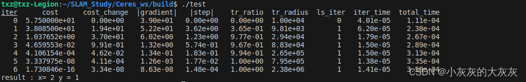
{ x 2 + y − 5 = 0 x + y − 3 = 0 4 x + y 2 − 9 = 0 \begin{cases} x^2+y-5=0 \\ x +y - 3 =0\\ 4x+y^2-9=0 \end{cases} ⎩ ⎨ ⎧x2+y−5=0x+y−3=04x+y2−9=0 - 代码
源代码
CMakeLists.txt#include"ceres/ceres.h" using ceres::AutoDiffCostFunction; using ceres::CostFunction; using ceres::Problem; using ceres::Solver; using ceres::Solve; /* 简介:定义的非线性方程组合 实例化用法:nonline_fun func; 调用的方法:func(x, result); */ struct nonline_fun { template <typename T> bool operator()(const T* const x, T* residual) const { residual[1] = x[0]*x[0] + x[1] - T(5.0); residual[0] = x[0] + x[1] - T(3.0); residual[2] = T(4.0) * x[0] + x[1] * x[1] - T(9.0); return true; } }; int main() { Problem problem; /* 待优化参数,这里的[0,0]也是一个粗略解 */ double y[2]={0.0, 0.0}; /* 定义一个Ceres认可的残差函数,3:残差数量, 2:待优化的变量个数 */ CostFunction* cost_function = new AutoDiffCostFunction<nonline_fun, 3, 2>(new nonline_fun); /* 将优化问题中初始化,使用非线性函数、待优化的变量进行初始化 */ problem.AddResidualBlock(cost_function, NULL, y); /* 定义求解的算子, 最大迭代次数、迭代终止时的最小相对损失变化阈值、迭代终止的最小梯度(都是默认值,可以自己修改试试+)*/ Solver::Options options; options.minimizer_progress_to_stdout = true; options.max_num_iterations = 50; options.function_tolerance = 1e-8; options.gradient_tolerance = 1e-6; /* 开始求解 */ Solver::Summary summary; Solve(options, &problem, &summary); std::cout << summary.BriefReport() << "\n"; std::cout << "result : x= " << y[0] << " y = " << y[1] << "\n"; return 0; }cmake_minimum_required(VERSION 2.8) project(ceres_ws) find_package(Ceres REQUIRED) include_directories(${CERES_INCLUDE_DIRS}) add_executable(test src/demo.cpp) target_link_libraries(test ${CERES_LIBRARIES}) - 运行结果
2. 拟合数据
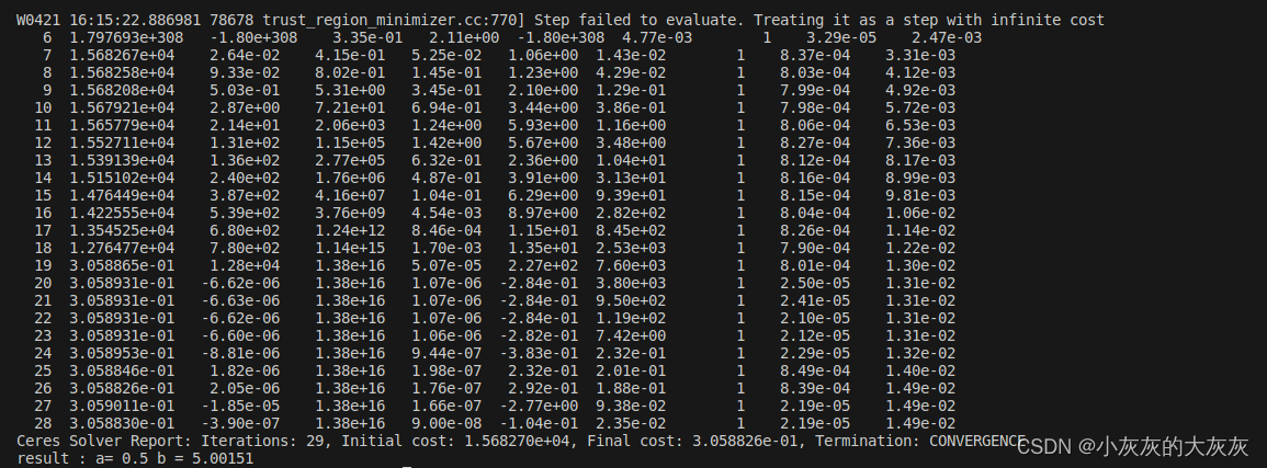
- 期望拟合的式子,在构造数据的时候指定了
a
=
0.5
,
b
=
5
a=0.5,b=5
a=0.5,b=5
y = e a x + 5 b y=e^{ax} + 5b y=eax+5b - 代码
#include<iostream> #include <vector> #include<random> #include<cmath> #include <algorithm> #include"ceres/ceres.h" using ceres::AutoDiffCostFunction; using ceres::CostFunction; using ceres::Problem; using ceres::Solver; using ceres::Solve; /* 待拟合的数据 */ std::vector<std::pair<double, double>> data_for_fitting; /* 简介:该函数产生用于拟合曲线的数据[(x, y)...], 默认产生1000组数据, 期望的函数: y = exp(ax) + bx ; a和b是未知数 */ void generate_data_for_fitting(int data_num=500){ /* 随机数的种子 */ std::default_random_engine e; /* 随机数的产生器 */ std::uniform_real_distribution<double> generate_random(-0.1, 0.2); /* 填充数据,并添加随机噪声 */ for (int i = 0; i < data_num; i++) { double value = exp(0.5*i) + 5*i + generate_random(e); data_for_fitting.push_back(std::make_pair(i, value)); } std::cout << "数据构造完成,共计数目:" << data_for_fitting.size() << std::endl; } /* 构建指数函数的残差, 构造函数用于初始化样本XY, 用法:ExponentialResidual(a, b, residual); */ struct ExponentialResidual { ExponentialResidual(double x, double y) : x_(x), y_(y) {} template <typename T> bool operator()(const T* const a, const T* const b, T* residual) const { residual[0] = y_ - (exp(a[0] * x_) + b[0]*x_ ); return true; } private: /* 样本的观察值 */ const double x_; const double y_; }; int main() { /* 生成数据到容器:data_for_fitting */ generate_data_for_fitting(); /* 构建最小二乘问题(argmin 0.5*||F(x)||**2 ) */ Problem problem; /* 待优化参数,这里的[0,0]也是一个粗略解 */ double a=0.0, b=0.0; /* 实际上就是添加了很多个方程, 为了程序的鲁棒性,添加了CauchyLoss(0.5) */ for (int i = 0; i < data_for_fitting.size(); ++i) { problem.AddResidualBlock( /* 参数1:定义的一个Ceres认可的残差函数,1(残差数量), 1:待优化的变量个数, 1:待优化的变量个数 */ new AutoDiffCostFunction<ExponentialResidual, 1, 1, 1>( new ExponentialResidual(data_for_fitting[i].first, data_for_fitting[i].second)), new ceres::CauchyLoss(0.5), &a, &b); } /*定义求解的算子, 最大迭代次数、迭代终止时的最小相对损失变化阈值、迭代终止的最小梯度(都是默认值,可以自己修改试试+) */ Solver::Options options; options.minimizer_progress_to_stdout = true; options.max_num_iterations = 50; options.linear_solver_type = ceres::DENSE_QR; options.function_tolerance = 1e-8; options.gradient_tolerance = 1e-6; /* 开始求解 */ Solver::Summary summary; Solve(options, &problem, &summary); std::cout << summary.BriefReport() << "\n"; std::cout << "result : a= " << a << " b = " << b << "\n"; return 0; } - 运行结果


 被折叠的 条评论
为什么被折叠?
被折叠的 条评论
为什么被折叠?
 到【灌水乐园】发言


