Towards Accurate One-Stage Object Detection with AP-Loss阅读笔记

Towards Accurate One-Stage Object Detection with AP-Loss

---

• 作者认为在one-stage的detection中，detection和classification任务之间的gap影响了模型的performance，于是把classification task改为ranking task，把classification loss 改为ranking loss，并采用APloss作为target loss
• 由于APloss是non-convex和non-differentiable，需要采取特殊的方法：

1. 用SVM来学习APloss
2. 修改loss为APloss的某个upper bound
3. approximate gradient methods
4. 论文提出的方法：改classification 为 ranking task，并使用一种error-driven的算法来optimize AP-loss，这里的error-driven的算法基于1957年提出的Perceptron Learning Algorithm，即采用sign函数作为activation function

• 我只是个莫得感情的论文搬运机器大意上是说原来的模型每个bbox输出k+1维向量而文章提出的模型只输出一个标量但是会重复k遍，而label也改为标量形式：

In our framework, instead of one box with K + 1 dimensional score predictions, we replicate each box bi for K times to obtain bik where k = 1, · · · , K, and the k-th box is responsible for the k-th class. Each box bik will be assigned a label tik ∈ {−1, 0, 1} through the same IoU strategy (label −1 for not counted into the ranking loss). Therefore, in the training and testing phase, the detector will predict only one scalar score sik for each box bik.

• 下面讲一下ap-loss的算法：

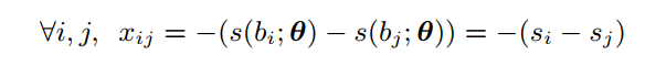
1. 既然anchor box的输出是一个标量（先不管重复输出），可以设为$b_i$，算得一个$x_{ij}$为两个anchor box之间差的度量，这里$s(b_i;\theta )$指模型参数为$\theta$的时候第i个anchor box的输出score：
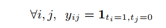
2. 同时需对label做类似的转换，表示$t_i=1，t_j=0$时$y_{ij}=1$否则为0，这里t就是label
   
3. primary-loss为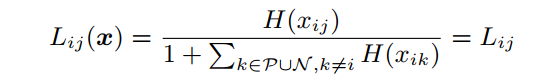：其中$H(x_{ij})$即前文所提的符号函数：
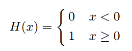
4. AP-loss为：其中$ran{k}^{+}(i)$为$s_i$在所有正样本中的排序值而$rank(i)$为$s_i$在所有有效样本中的排序值， P = { i ∣ t i = 1 } , N = { i ∣ t i = 0 } P = \left\{ i|t_i = 1\right\}, N = \left\{i|t_i = 0\right\} P={i∣ti​=1},N={i∣ti​=0}，L and y are vector form for all $L_{ij}$ and $y_{ij}$ respectively, <, >means dot-product of two input vectors.注意 x，y，L都是d维向量，d为有效输出的anchor数。
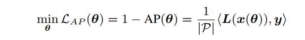5. 所以optimize的目标为为但这里的L是不可导的，需要采用特殊的方法
6. Perceptron Learning Algorithm是这样的：

Suppose $x_{ij}$ is the input and $L_{ij}$ is the current output, the update for $x_{ij}$ is thus $$∆x_{ij}=L_{ij}^{\ast }-L_{ij}$$ where $L_{ij}^{\ast }$ is the desired output.

7. 而论文的error-driven算法是这样的：

$$∆x_{ij}=-L_{ij}\cdot y_{ij}$$

从loss的形式可以看出，当L·y为0时有最小的loss，而有两种情况，一种y为0，则L不论多少都没关系此时不更新，一种y为1则L期望为0，所以采取这样的更新形式

8.方向传播对于$s_i$的gradient的形式是这样的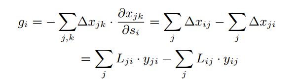：实践中即设一个$x_{ij}$ 的梯度为 $-∆x_{ij}$，至于为什么是这种形式，论文中给出了推导，也不复杂，这里就不赘诉。

训练细节：

• minibatch可以应用到AP-loss的ranking中
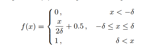
• 前期训练由于$s_i$差距很小会导致较大的loss，训练不稳定，可以H(·)函数为

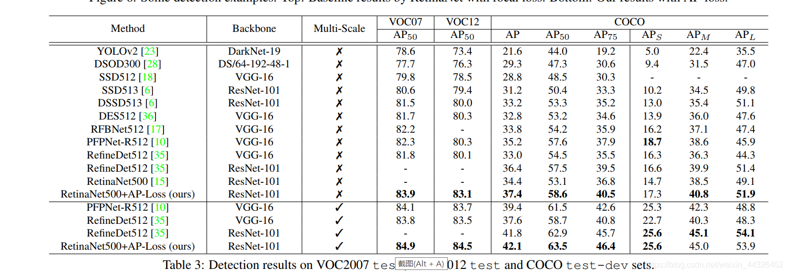
experiment