


连续类功放通解2:连续类单管功率放大器底层实现原理
本次内容理论性较强,适合对功率放大器理论研究比较感兴趣以及想发论文的小朋友,着重探讨现有的一些带宽拓展模式(也就是连续类)的基本实现原理,并给出其通用的分析求解方法。
前置介绍:
连续类功放通解1:连续类单管功率放大器现有理论
0、思路与直觉
连续类功率放大器能够在不牺牲效率的情况下拓展带宽,因此得到的广泛的研究。从数学角度去理解,连续模式的宽带设计空间(以及其对应的波形)实际上就是一个恒定效率方程的解。
0.1简单回顾
功率放大器的Smith圆图(频域)上的设计空间和其时域波形直接相关,如连续类功放通解1:连续类单管功率放大器现有理论文章中所给出的计算公式那样(基于原始电压电流波形的傅里叶分量,使用阻抗求解公式进行各次阻抗的求解):
V
d
s
(
θ
)
=
a
V
,
0
2
+
∑
n
=
1
∞
a
V
,
n
cos
(
n
θ
)
+
∑
n
=
1
∞
b
V
,
n
sin
(
n
θ
)
a
V
,
0
=
2
\begin{aligned} & V_{ds}(\theta)=\frac{a_{V, 0}}{2}+\sum_{n=1}^{\infty} a_{V, n} \cos (n \theta)+\sum_{n=1}^{\infty} b_{V, n} \sin (n \theta) \\ & a_{V, 0}=2 \end{aligned}
Vds(θ)=2aV,0+n=1∑∞aV,ncos(nθ)+n=1∑∞bV,nsin(nθ)aV,0=2
I
d
s
(
θ
)
=
a
I
,
0
2
+
∑
n
=
1
∞
a
I
,
n
cos
(
n
θ
)
+
∑
n
=
1
∞
b
I
,
n
sin
(
n
θ
)
a
I
,
0
=
2
\begin{aligned} & I_{ds}(\theta)=\frac{a_{I, 0}}{2}+\sum_{n=1}^{\infty} a_{I, n} \cos (n \theta)+\sum_{n=1}^{\infty} b_{I, n} \sin (n \theta) \\ & a_{I, 0}=2 \end{aligned}
Ids(θ)=2aI,0+n=1∑∞aI,ncos(nθ)+n=1∑∞bI,nsin(nθ)aI,0=2
Z
n
f
=
−
a
V
c
,
n
(
β
)
+
j
b
V
c
,
n
(
β
)
a
I
,
n
+
j
b
I
,
n
{Z_{nf}} = - \frac{{{a_{Vc,n}}(\beta ) + j{b_{Vc,n}}(\beta )}}{{{a_{I,n}} + j{b_{I,n}}}}
Znf=−aI,n+jbI,naVc,n(β)+jbVc,n(β)
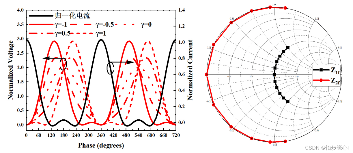
因此,所有的带宽拓展模式的直观解释就是因为时域波形的拓展,由此导致了频域设计空间由单点变成连续的线段,由此实现了宽带性能。
那么连续类功率放大器牺牲了什么呢?连续类PA的波形的峰值在不同阻抗条件下不固定,峰值大的波形易出现击穿,这是其主要的劣质,可参考下图中的电压峰值在2-3倍Vcc之间变化(连续B/J类波形与相应的宽带空间):
1、恒定高效率方程
之前提及,从数学角度去理解,连续模式的宽带设计空间(以及其对应的波形)实际上就是一个恒定效率方程的解。找到这个方程非常有意义,因为这样的方程可以应用于所有的波形,并有潜力给出任意波形的连续拓展模式。
在此给出这个理想的恒定效率方程的直接表达,其主要包含下面两个约束:
- 基波输出效率为𝜂
- 谐波不消耗功率
基于0.1简单回顾小节中的傅里叶分解假设,将上面的方程转化为数学形式,如下所示:
η
=
P
1
f
P
i
n
=
−
a
I
,
1
a
V
c
,
1
+
b
I
,
1
b
V
c
,
1
2
P
i
n
P
n
f
=
−
a
I
,
n
a
V
c
,
n
+
b
I
,
n
b
V
c
,
n
2
=
0
(
n
>
1
)
\begin{aligned} &\eta = \frac{{{P_{1f}}}}{{{P_{in}}}} = - \frac{{{a_{I,1}}{a_{Vc,1}} + {b_{I,1}}{b_{Vc,1}}}}{{2{P_{in}}}}\\ &{P_{nf}} = - \frac{{{a_{I,n}}{a_{Vc,n}} + {b_{I,n}}{b_{Vc,n}}}}{2} = 0(n>1) \end{aligned}
η=PinP1f=−2PinaI,1aVc,1+bI,1bVc,1Pnf=−2aI,naVc,n+bI,nbVc,n=0(n>1)
P
i
n
=
V
D
C
⋅
I
D
C
=
a
I
,
0
2
⋅
a
V
c
,
0
2
\begin{aligned} & {P_{in}} = {V_{DC}} \cdot {I_{DC}} = \frac{{{a_{I,0}}}}{2} \cdot \frac{{{a_{Vc,0}}}}{2} \end{aligned}
Pin=VDC⋅IDC=2aI,0⋅2aVc,0
简单验证连续F类是否满足上面的方程,连续F类的波形表达式如下所示:
V
C
F
=
(
1
−
2
3
cos
θ
)
2
⋅
(
1
+
1
3
cos
θ
)
⋅
(
1
−
γ
sin
θ
)
=
1
−
2
3
cos
θ
−
γ
sin
θ
+
7
γ
6
3
sin
2
θ
+
1
3
3
cos
3
θ
−
7
γ
6
3
cos
4
θ
I
C
F
=
1
π
+
1
2
cos
θ
+
2
3
π
cos
(
2
θ
)
\begin{aligned} &{V_{CF}} = {\left( {1 - \frac{2}{{\sqrt 3 }}\cos \theta } \right)^2} \cdot \left( {1 + \frac{1}{{\sqrt 3 }}\cos \theta } \right) \cdot (1 - \gamma \sin \theta )\\ &{\rm{ = 1}} - \frac{2}{{\sqrt 3 }}\cos \theta - \gamma \sin \theta {\rm{ + }}\frac{{{\rm{7}}\gamma }}{{{\rm{6}}\sqrt 3 }}\sin {\rm{2}}\theta {\rm{ + }}\frac{{\rm{1}}}{{{\rm{3}}\sqrt 3 }}\cos 3\theta - \frac{{{\rm{7}}\gamma }}{{{\rm{6}}\sqrt 3 }}\cos 4\theta \\ &{I_{CF}} = \frac{1}{\pi } + \frac{1}{2}\cos \theta + \frac{2}{{3\pi }}\cos (2\theta ) \end{aligned}
VCF=(1−32cosθ)2⋅(1+31cosθ)⋅(1−γsinθ)=1−32cosθ−γsinθ+637γsin2θ+331cos3θ−637γcos4θICF=π1+21cosθ+3π2cos(2θ)
基于上面的傅里叶分量对效率进行计算,可得:
P
1
f
=
−
a
I
,
1
a
V
,
1
+
b
I
,
1
b
V
,
1
2
=
−
1
2
×
(
−
2
3
)
+
0
×
(
−
γ
)
2
=
1
2
3
P
n
f
=
−
a
I
,
n
a
V
,
n
+
b
I
,
n
b
V
,
n
2
=
0
(
n
>
1
)
η
=
P
1
f
P
i
n
=
1
2
3
1
π
≈
0.907
\begin{aligned} &{P_{1f}} = - \frac{{{a_{I,1}}{a_{V,1}} + {b_{I,1}}{b_{V,1}}}}{2} = - \frac{{\frac{1}{2} \times \left( { - \frac{2}{{\sqrt 3 }}} \right) + 0 \times \left( { - \gamma } \right)}}{2} = \frac{1}{{2\sqrt 3 }}\\ &{P_{nf}} = - \frac{{{a_{I,n}}{a_{V,n}} + {b_{I,n}}{b_{V,n}}}}{2} = 0(n > 1)\\ &\eta = \frac{{{P_{1f}}}}{{{P_{in}}}} = \frac{{\frac{1}{{2\sqrt 3 }}}}{{\frac{1}{\pi }}} \approx 0.907 \end{aligned}
P1f=−2aI,1aV,1+bI,1bV,1=−221×(−32)+0×(−γ)=231Pnf=−2aI,naV,n+bI,nbV,n=0(n>1)η=PinP1f=π1231≈0.907
由此可见,虽然连续F类在连续F类的基础上乘以了
(
1
−
γ
sin
(
θ
)
)
(1 - \gamma \sin (\theta ))
(1−γsin(θ)),但是最终的效率结果和
γ
\gamma
γ无关,由此在维持效率不变的同时拓展了波形,由此拓展了宽带的设计空间。
2、如何对波形进行拓展
上面的分析是一个正向的过程,我们已知了连续因子 ( 1 − γ sin ( θ ) ) (1 - \gamma \sin (\theta )) (1−γsin(θ)),并使用得到的一簇波形解带入方程进行分析,最终发现其满足恒定效率方程。
实际上,如果知道原始的波形,我们也可以通过方程的求解来解得这个连续因子。如果我们能够使用这样的思路进行求解,我们自然能够将这样的方法拓展到任意的波形中去。打个简单的例子,我们事先知道了F类的电流和电压波形,我们如何求解出 ( 1 − γ sin ( θ ) ) (1 - \gamma \sin (\theta )) (1−γsin(θ))呢?在此简单介绍。
我们不知道乘以什么样的连续因子才能实现带宽的拓展,因此我们需要将连续因子F设为傅里叶分解的形式:
F
(
θ
,
β
)
=
a
F
v
,
0
(
β
)
2
+
∑
n
=
1
∞
a
F
v
,
n
(
β
)
cos
(
n
θ
)
+
∑
n
=
1
∞
b
F
v
,
n
(
β
)
sin
(
n
θ
)
F(\theta,\beta)=\frac{a_{F v, 0}(\beta)}{2}+\sum_{n=1}^{\infty} a_{F v, n}(\beta) \cos (n \theta)+\sum_{n=1}^{\infty} b_{F v, n}(\beta) \sin (n \theta)
F(θ,β)=2aFv,0(β)+n=1∑∞aFv,n(β)cos(nθ)+n=1∑∞bFv,n(β)sin(nθ)
相应的,将原始的归一化波形和连续因子相乘,可以得到连续波形
V
d
−
c
(
θ
,
β
)
V_{d_{-} c}(\theta,\beta)
Vd−c(θ,β):
V
d
−
c
(
θ
,
β
)
=
V
d
−
n
(
θ
)
⋅
F
(
θ
,
β
)
V_{d_{-} c}(\theta,\beta)=V_{d_{-} n}(\theta) \cdot F(\theta,\beta)
Vd−c(θ,β)=Vd−n(θ)⋅F(θ,β)
对于此处得到的连续波形
V
d
−
c
(
θ
,
β
)
V_{d_{-} c}(\theta,\beta)
Vd−c(θ,β),我们也可以将其写为傅里叶分解的形式:
V
d
−
c
(
θ
,
β
)
=
a
V
c
,
0
2
+
∑
n
=
1
∞
(
a
V
c
,
n
cos
(
n
θ
)
+
b
V
c
,
n
sin
(
n
θ
)
)
V_{d_{-} c}(\theta,\beta)=\frac{a_{V c, 0}}{2}+\sum_{n=1}^{\infty} \left(a_{V c, n} \cos (n \theta)+b_{V c, n} \sin (n \theta)\right)
Vd−c(θ,β)=2aVc,0+n=1∑∞(aVc,ncos(nθ)+bVc,nsin(nθ))
连续波形
V
d
−
c
(
θ
,
β
)
V_{d_{-} c}(\theta,\beta)
Vd−c(θ,β)的傅里叶分量一定会满足恒定效率方程,由此可以构建方程组。到此为止,需要强调的是,我们的未知数只有连续因子F的傅里叶分量,其余的一切都是已知的(例如初始电压、电流波形的傅里叶分量等等)。
在实际分析时,我们都是最多考虑到5次谐波,因此实际的未知量有11个,就是连续因子F的傅里叶分量(5个正弦分量、5个余弦分量、1个直流分量),但是我们的恒定效率方程只有五个,这意味着方程组的解并不唯一。如何直观的理解这个含义呢,下面我们举例介绍。
假设我们对F类的波形使用上面的方法进行求解,我们假设了一个连续因子F,我们会得到下面这样的线性方程组:
M
−
C
⋅
M
−
F
v
=
[
M
−
c
1
f
M
−
c
2
f
M
−
c
3
f
M
−
c
4
f
M
−
c
5
f
]
⋅
M
−
F
v
=
0
M_{-} C \cdot M_{-} F_v=\left[\begin{array}{l} M_{-} c_{1 f} \\ M_{-} c_{2 f} \\ M_{-} c_{3 f} \\ M_{-} c_{4 f} \\ M_{-} c_{5 f} \end{array}\right] \cdot M_{-} F_v=0
M−C⋅M−Fv=
M−c1fM−c2fM−c3fM−c4fM−c5f
⋅M−Fv=0
其中
M
−
F
v
M_{-} F_v
M−Fv是连续因子F的傅里叶分量,在考虑5次谐波时一共有11个,
M
−
c
n
f
M_{-} c_{n f}
M−cnf为第n个方程的系数,我们假设的未知数只有连续因子F的傅里叶分量,因此
M
−
c
n
f
M_{-} c_{n f}
M−cnf也是已知的。
M
−
F
v
=
[
a
F
v
,
0
a
F
v
,
1
a
F
v
,
2
a
F
v
,
3
a
F
v
,
4
a
F
v
,
5
b
F
v
,
1
b
F
v
,
2
b
F
v
,
3
b
F
v
,
4
b
F
v
,
5
]
T
M
−
c
n
f
=
[
c
n
f
a
,
0
c
n
f
a
,
1
c
n
f
a
,
2
c
n
f
a
,
3
c
n
f
a
,
4
c
n
f
a
,
5
c
n
f
b
,
1
c
n
f
b
,
2
c
n
f
b
,
3
c
n
f
b
,
4
c
n
f
b
,
5
]
\begin{aligned} &M_{-} F_v=\left[\begin{array}{lllllllllll} a_{Fv,{0} } & a_{Fv,{1} } & a_{Fv,{2} } & a_{Fv,{3} } & a_{Fv,{4} } & a_{Fv,{5} } & b_{Fv,{1} } & b_{Fv,{2} } & b_{Fv,{3} } & b_{Fv,{4} } & b_{Fv,{5} } \end{array}\right]^T\\ &M_{-} c_{n f}=\left[\begin{array}{lllllllllll} c_{nf a, 0} & c_{nf a, 1} & c_{nf a, 2} & c_{nf a, 3} & c_{nf a, 4} & c_{nf a, 5} & c_{nf b, 1} & c_{nf b, 2} & c_{nf b, 3} & c_{nf b, 4} & c_{nf b, 5}\\ \end{array}\right]\\ \end{aligned}
M−Fv=[aFv,0aFv,1aFv,2aFv,3aFv,4aFv,5bFv,1bFv,2bFv,3bFv,4bFv,5]TM−cnf=[cnfa,0cnfa,1cnfa,2cnfa,3cnfa,4cnfa,5cnfb,1cnfb,2cnfb,3cnfb,4cnfb,5]
实际的未知量有11个,恒定效率方程只有五个,方程组一定有多组解,我们需要对方程组的通解进行求取。对于连续F类,我们必定可以解得恒定效率方程的通解一定包含以下两个:
M
−
F
0
=
[
2
0
0
0
0
0
0
0
0
0
0
]
T
M
−
F
1
=
[
0
0
0
0
0
0
1
0
0
0
0
]
T
\begin{aligned} &M_{-} F_0=\left[\begin{array}{lllllllllll} 2 & 0 & 0 & 0 & 0 & 0 & 0 & 0 & 0 & 0 & 0 \end{array}\right]^T\\ &M_{-} F_1=\left[\begin{array}{lllllllllll} 0 & 0 & 0 & 0 & 0 & 0 & 1 & 0 & 0 & 0 & 0 \end{array}\right]^T\\ \end{aligned}
M−F0=[20000000000]TM−F1=[00000010000]T
使用线性代数的知识,我们必知
M
−
F
0
−
β
M
−
F
1
M_{-} F_0- \beta M_{-} F_1
M−F0−βM−F1也是方程组的解,因此得到一组解为:
M
−
F
v
=
[
2
0
0
0
0
0
−
β
0
0
0
0
]
T
\begin{aligned} &M_{-} F_v=\left[\begin{array}{lllllllllll} 2 & 0 & 0 & 0 & 0 & 0 & -\beta & 0 & 0 & 0 & 0 \end{array}\right]^T\\ \end{aligned}
M−Fv=[200000−β0000]T
这样我们就可以得到连续F类的一个连续因子:
F
(
θ
,
β
)
=
a
F
v
,
0
(
β
)
2
+
∑
n
=
1
∞
a
F
v
,
n
(
β
)
cos
(
n
θ
)
+
∑
n
=
1
∞
b
F
v
,
n
(
β
)
sin
(
n
θ
)
=
(
1
−
β
sin
(
θ
)
)
F(\theta,\beta)=\frac{a_{F v, 0}(\beta)}{2}+\sum_{n=1}^{\infty} a_{F v, n}(\beta) \cos (n \theta)+\sum_{n=1}^{\infty} b_{F v, n}(\beta) \sin (n \theta)=(1 - \beta\sin (\theta ))
F(θ,β)=2aFv,0(β)+n=1∑∞aFv,n(β)cos(nθ)+n=1∑∞bFv,n(β)sin(nθ)=(1−βsin(θ))
这边还有一个细节问题,就是
M
−
F
0
、
M
−
F
1
M_{-} F_0、 M_{-} F_1
M−F0、M−F1是方程的通解,那么
F
(
θ
,
β
)
=
1
、
2
、
3
、
4......
F(\theta,\beta)=1、2、3、4......
F(θ,β)=1、2、3、4......以及
F
(
θ
,
β
)
=
s
i
n
(
θ
)
、
2
s
i
n
(
θ
)
、
3
s
i
n
(
θ
)
、
4
s
i
n
(
θ
)
.
.
.
.
.
.
F(\theta,\beta)=sin(\theta)、2sin(\theta)、3sin(\theta)、4sin(\theta)......
F(θ,β)=sin(θ)、2sin(θ)、3sin(θ)、4sin(θ)......应该都能满足拓展的要求,但是在实际过程中,我们需要要求被拓展后得到的波形的直流分量保持不变(供电电压总是不变的),因此乘以了这些数之后还需要进行重新的归一化。只乘以
s
i
n
(
θ
)
sin(\theta)
sin(θ)也是同理。
而单独乘以
s
i
n
(
θ
)
sin(\theta)
sin(θ)会导致直流分量消失,得到无解,我们需要将
s
i
n
(
θ
)
sin(\theta)
sin(θ)看成
S
+
s
i
n
(
θ
)
S+sin(\theta)
S+sin(θ),其中S为无穷小:
V
C
F
=
(
1
−
2
3
cos
θ
)
2
⋅
(
1
+
1
3
cos
θ
)
⋅
(
S
−
γ
sin
θ
)
=
S
−
2
3
S
cos
θ
−
γ
sin
θ
+
7
γ
6
3
sin
2
θ
+
1
3
3
S
cos
3
θ
−
7
γ
6
3
cos
4
θ
I
C
F
=
1
π
+
1
2
cos
θ
+
2
3
π
cos
(
2
θ
)
\begin{aligned} &{V_{CF}} = {\left( {1 - \frac{2}{{\sqrt 3 }}\cos \theta } \right)^2} \cdot \left( {1 + \frac{1}{{\sqrt 3 }}\cos \theta } \right) \cdot (S - \gamma \sin \theta )\\ &{{ = S}} - \frac{2}{{\sqrt 3 }}S\cos \theta - \gamma \sin \theta {\rm{ + }}\frac{{{\rm{7}}\gamma }}{{{\rm{6}}\sqrt 3 }}\sin {\rm{2}}\theta {\rm{ + }}\frac{{\rm{1}}}{{{\rm{3}}\sqrt 3 }}S\cos 3\theta - \frac{{{\rm{7}}\gamma }}{{{\rm{6}}\sqrt 3 }}\cos 4\theta \\ &{I_{CF}} = \frac{1}{\pi } + \frac{1}{2}\cos \theta + \frac{2}{{3\pi }}\cos (2\theta ) \end{aligned}
VCF=(1−32cosθ)2⋅(1+31cosθ)⋅(S−γsinθ)=S−32Scosθ−γsinθ+637γsin2θ+331Scos3θ−637γcos4θICF=π1+21cosθ+3π2cos(2θ)
结合高数中等价无穷小的知识进行化简,得到如下结果:
P
1
f
=
−
a
I
,
1
a
V
,
1
+
b
I
,
1
b
V
,
1
2
=
−
1
2
×
(
−
2
3
S
)
+
0
×
(
−
γ
)
2
=
S
2
3
P
n
f
=
−
a
I
,
n
a
V
,
n
+
b
I
,
n
b
V
,
n
2
=
0
(
n
>
1
)
η
=
P
1
f
P
i
n
=
S
2
3
S
π
≈
0.907
\begin{aligned} &{P_{1f}} = - \frac{{{a_{I,1}}{a_{V,1}} + {b_{I,1}}{b_{V,1}}}}{2} = - \frac{{\frac{1}{2} \times \left( { - \frac{2}{{\sqrt 3 }}}S \right) + 0 \times \left( { - \gamma } \right)}}{2} = \frac{S}{{2\sqrt 3 }}\\ &{P_{nf}} = - \frac{{{a_{I,n}}{a_{V,n}} + {b_{I,n}}{b_{V,n}}}}{2} = 0(n > 1)\\ &\eta = \frac{{{P_{1f}}}}{{{P_{in}}}} = \frac{{\frac{S}{{2\sqrt 3 }}}}{{\frac{S}{\pi }}} \approx 0.907 \end{aligned}
P1f=−2aI,1aV,1+bI,1bV,1=−221×(−32S)+0×(−γ)=23SPnf=−2aI,naV,n+bI,nbV,n=0(n>1)η=PinP1f=πS23S≈0.907
3、恒定高效率方程的求解
简要的思路在上一小节中已经介绍过了,详细的推导过程可以参考下面的论文:
A continuous Class-EF power amplifier based on the general continuous mode design theory
计算过程相对复杂,此处给出Matlab代码来帮助大家实际分析求解。
%计算基底
clc
clear all
syms afv0 afv1 afv2 afv3 afv4 afv5 bfv1 bfv2 bfv3 bfv4 bfv5
% 初始化F类波形的傅里叶分量
Vds_fouier=[1,-2/sqrt(3),0,1/(3*sqrt(3)),0,0,0,0,0,0,0];
Ids_fouier=pi*[1/pi,0.5,2/(3*pi),0,0,0,0,0,0,0,0];


av0=Vds_fouier(1)*2;av1=Vds_fouier(2);av2=Vds_fouier(3);av3=Vds_fouier(4);av4=Vds_fouier(5);av5=Vds_fouier(6);
bv1=Vds_fouier(7);bv2=Vds_fouier(8);bv3=Vds_fouier(9);bv4=Vds_fouier(10);bv5=Vds_fouier(11);
ai0=Ids_fouier(1)*2;ai1=Ids_fouier(2);ai2=Ids_fouier(3);ai3=Ids_fouier(4);ai4=Ids_fouier(5);ai5=Ids_fouier(6);
bi1=Ids_fouier(7);bi2=Ids_fouier(8);bi3=Ids_fouier(9);bi4=Ids_fouier(10);bi5=Ids_fouier(11);
eta=-(ai1*av1+bi1*bv1)/2/(av0/2*ai0/2);

c_afv0=(ai1*av1)/4 + (bi1*bv1)/4 + (av0*eta)/4;
c_afv1=(bi1*bv2)/4 + (av1*eta)/2 + (ai1*(av0/2 + av2/2))/2;
c_afv2=(av2*eta)/2 + (ai1*(av1/2 + av3/2))/2 - (bi1*(bv1/2 - bv3/2))/2;
c_afv3=(av3*eta)/2 + (ai1*(av2/2 + av4/2))/2 - (bi1*(bv2/2 - bv4/2))/2;
c_afv4=(av4*eta)/2 + (ai1*(av3/2 + av5/2))/2 - (bi1*(bv3/2 - bv5/2))/2;
c_afv5=(ai1*av4)/4 - (bi1*bv4)/4 + (av5*eta)/2;
c_bfv1=(ai1*bv2)/4 + (bv1*eta)/2 + (bi1*(av0/2 - av2/2))/2;
c_bfv2=(bv2*eta)/2 + (bi1*(av1/2 - av3/2))/2 + (ai1*(bv1/2 + bv3/2))/2;
c_bfv3=(bv3*eta)/2 + (bi1*(av2/2 - av4/2))/2 + (ai1*(bv2/2 + bv4/2))/2;
c_bfv4=(bv4*eta)/2 + (bi1*(av3/2 - av5/2))/2 + (ai1*(bv3/2 + bv5/2))/2;
c_bfv5=(ai1*bv4)/4 + (av4*bi1)/4 + (bv5*eta)/2;
coff_1nd=[c_afv0 c_afv1 c_afv2 c_afv3 c_afv4 c_afv5 c_bfv1 c_bfv2 c_bfv3 c_bfv4 c_bfv5];

c_afv0=(ai2*av2)/2 + (bi2*bv2)/2;
c_afv1=ai2*(av1/2 + av3/2) + bi2*(bv1/2 + bv3/2);
c_afv2=(bi2*bv4)/2 + ai2*(av0/2 + av4/2);
c_afv3=ai2*(av1/2 + av5/2) - bi2*(bv1/2 - bv5/2);
c_afv4=(ai2*av2)/2 - (bi2*bv2)/2;
c_afv5=(ai2*av3)/2 - (bi2*bv3)/2;
c_bfv1=bi2*(av1/2 - av3/2) - ai2*(bv1/2 - bv3/2);
c_bfv2=(ai2*bv4)/2 + bi2*(av0/2 - av4/2);
c_bfv3=bi2*(av1/2 - av5/2) + ai2*(bv1/2 + bv5/2);
c_bfv4=(ai2*bv2)/2 + (av2*bi2)/2;
c_bfv5=(ai2*bv3)/2 + (av3*bi2)/2;
coff_2nd=[c_afv0 c_afv1 c_afv2 c_afv3 c_afv4 c_afv5 c_bfv1 c_bfv2 c_bfv3 c_bfv4 c_bfv5];

c_afv0=(ai3*av3)/2 + (bi3*bv3)/2;
c_afv1=ai3*(av2/2 + av4/2) + bi3*(bv2/2 + bv4/2);
c_afv2=ai3*(av1/2 + av5/2) + bi3*(bv1/2 + bv5/2);
c_afv3=(ai3*av0)/2;
c_afv4=(ai3*av1)/2 - (bi3*bv1)/2;
c_afv5=(ai3*av2)/2 - (bi3*bv2)/2;
c_bfv1=bi3*(av2/2 - av4/2) - ai3*(bv2/2 - bv4/2);
c_bfv2=bi3*(av1/2 - av5/2) - ai3*(bv1/2 - bv5/2);
c_bfv3=(av0*bi3)/2;
c_bfv4=(ai3*bv1)/2 + (av1*bi3)/2;
c_bfv5=(ai3*bv2)/2 + (av2*bi3)/2;
coff_3nd=[c_afv0 c_afv1 c_afv2 c_afv3 c_afv4 c_afv5 c_bfv1 c_bfv2 c_bfv3 c_bfv4 c_bfv5];

c_afv0=(ai4*av4)/2 + (bi4*bv4)/2;
c_afv1=ai4*(av3/2 + av5/2) + bi4*(bv3/2 + bv5/2);
c_afv2=(ai4*av2)/2 + (bi4*bv2)/2;
c_afv3=(ai4*av1)/2 + (bi4*bv1)/2;
c_afv4=(ai4*av0)/2;
c_afv5=(ai4*av1)/2 - (bi4*bv1)/2;
c_bfv1=bi4*(av3/2 - av5/2) - ai4*(bv3/2 - bv5/2);
c_bfv2=(av2*bi4)/2 - (ai4*bv2)/2;
c_bfv3=(av1*bi4)/2 - (ai4*bv1)/2;
c_bfv4=(av0*bi4)/2;
c_bfv5=(ai4*bv1)/2 + (av1*bi4)/2;
coff_4nd=[c_afv0 c_afv1 c_afv2 c_afv3 c_afv4 c_afv5 c_bfv1 c_bfv2 c_bfv3 c_bfv4 c_bfv5];

c_afv0=(ai5*av5)/2 + (bi5*bv5)/2;
c_afv1=(ai5*av4)/2 + (bi5*bv4)/2;
c_afv2=(ai5*av3)/2 + (bi5*bv3)/2;
c_afv3=(ai5*av2)/2 + (bi5*bv2)/2;
c_afv4=(ai5*av1)/2 + (bi5*bv1)/2;
c_afv5=(ai5*av0)/2;
c_bfv1=(av4*bi5)/2 - (ai5*bv4)/2;
c_bfv2=(av3*bi5)/2 - (ai5*bv3)/2;
c_bfv3=(av2*bi5)/2 - (ai5*bv2)/2;
c_bfv4=(av1*bi5)/2 - (ai5*bv1)/2;
c_bfv5=(av0*bi5)/2;
coff_5nd=[c_afv0 c_afv1 c_afv2 c_afv3 c_afv4 c_afv5 c_bfv1 c_bfv2 c_bfv3 c_bfv4 c_bfv5];

matrix_coff=zeros(11,11);
matrix_coff(1,1:11)=coff_1nd;
matrix_coff(2,1:11)=coff_2nd;
matrix_coff(3,1:11)=coff_3nd;
matrix_coff(4,1:11)=coff_4nd;
matrix_coff(5,1:11)=coff_5nd;

[m,n]=eig(matrix_coff);


b1=1;
b2=8;
beta1=m(:,b1);
% beta1=m(:,b1);
beta2=m(:,b2)-beta1*(m(:,b2)'*beta1)/(beta1'*beta1);

disp(['正交特征向量1为:'])
disp(num2str(beta1'))
disp(['正交特征向量2为:'])
disp(num2str(beta2'))
disp('-------------------------------------------------------------------------------------------------------------------------------')

lamda = sym('lamda','real');
fv_arrary=beta1+lamda*beta2;
fv_arrary(1)=fv_arrary(1);
tmp=simplify(sum(fv_arrary'.*Vds_fouier));
disp(['Norm Factor is:'])
disp(tmp);
disp('-------------------------------------------------------------------------------------------------------------------------------')
%对得出的波形进行验证,验证要求是关于虚轴对称分布
beta = sym('beta','real');
fv_arrary_tmp1=beta1;
fv_arrary_tmp2=beta2;
fv_arrary=fv_arrary_tmp1+fv_arrary_tmp2*beta;
afv0=fv_arrary(1);afv1=fv_arrary(2);afv2=fv_arrary(3);afv3=fv_arrary(4);afv4=fv_arrary(5);afv5=fv_arrary(6);
bfv1=fv_arrary(7);bfv2=fv_arrary(8);bfv3=fv_arrary(9);bfv4=fv_arrary(10);bfv5=fv_arrary(11);

avc0=(afv0*av0)/4 + (afv1*av1)/2 + (afv2*av2)/2 + (afv3*av3)/2 + (afv4*av4)/2 + (afv5*av5)/2 + (bfv1*bv1)/2 + (bfv2*bv2)/2 + (bfv3*bv3)/2 + (bfv4*bv4)/2 + (bfv5*bv5)/2;
avc1=(afv0*av1)/2 + (afv1*av0)/2 + (afv1*av2)/2 + (afv2*av1)/2 + (afv2*av3)/2 + (afv3*av2)/2 + (afv3*av4)/2 + (afv4*av3)/2 + (afv4*av5)/2 + (afv5*av4)/2 + (bfv1*bv2)/2 + (bfv2*bv1)/2 + (bfv2*bv3)/2 + (bfv3*bv2)/2 + (bfv3*bv4)/2 + (bfv4*bv3)/2 + (bfv4*bv5)/2 + (bfv5*bv4)/2;
bvc1=(afv0*bv1)/2 + (av0*bfv1)/2 + (afv1*bv2)/2 - (afv2*bv1)/2 + (av1*bfv2)/2 - (av2*bfv1)/2 + (afv2*bv3)/2 - (afv3*bv2)/2 + (av2*bfv3)/2 - (av3*bfv2)/2 + (afv3*bv4)/2 - (afv4*bv3)/2 + (av3*bfv4)/2 - (av4*bfv3)/2 + (afv4*bv5)/2 - (afv5*bv4)/2 + (av4*bfv5)/2 - (av5*bfv4)/2;
avc2=(afv0*av2)/2 + (afv1*av1)/2 + (afv2*av0)/2 + (afv1*av3)/2 + (afv3*av1)/2 + (afv2*av4)/2 + (afv4*av2)/2 + (afv3*av5)/2 + (afv5*av3)/2 - (bfv1*bv1)/2 + (bfv1*bv3)/2 + (bfv3*bv1)/2 + (bfv2*bv4)/2 + (bfv4*bv2)/2 + (bfv3*bv5)/2 + (bfv5*bv3)/2;
bvc2=(afv0*bv2)/2 + (afv1*bv1)/2 + (av0*bfv2)/2 + (av1*bfv1)/2 + (afv1*bv3)/2 - (afv3*bv1)/2 + (av1*bfv3)/2 - (av3*bfv1)/2 + (afv2*bv4)/2 - (afv4*bv2)/2 + (av2*bfv4)/2 - (av4*bfv2)/2 + (afv3*bv5)/2 - (afv5*bv3)/2 + (av3*bfv5)/2 - (av5*bfv3)/2;
avc3=(afv0*av3)/2 + (afv1*av2)/2 + (afv2*av1)/2 + (afv3*av0)/2 + (afv1*av4)/2 + (afv4*av1)/2 + (afv2*av5)/2 + (afv5*av2)/2 - (bfv1*bv2)/2 - (bfv2*bv1)/2 + (bfv1*bv4)/2 + (bfv4*bv1)/2 + (bfv2*bv5)/2 + (bfv5*bv2)/2;
bvc3=(afv0*bv3)/2 + (afv1*bv2)/2 + (afv2*bv1)/2 + (av0*bfv3)/2 + (av1*bfv2)/2 + (av2*bfv1)/2 + (afv1*bv4)/2 - (afv4*bv1)/2 + (av1*bfv4)/2 - (av4*bfv1)/2 + (afv2*bv5)/2 - (afv5*bv2)/2 + (av2*bfv5)/2 - (av5*bfv2)/2;
avc4=(afv0*av4)/2 + (afv1*av3)/2 + (afv2*av2)/2 + (afv3*av1)/2 + (afv4*av0)/2 + (afv1*av5)/2 + (afv5*av1)/2 - (bfv1*bv3)/2 - (bfv2*bv2)/2 - (bfv3*bv1)/2 + (bfv1*bv5)/2 + (bfv5*bv1)/2;
bvc4=(afv0*bv4)/2 + (afv1*bv3)/2 + (afv2*bv2)/2 + (afv3*bv1)/2 + (av0*bfv4)/2 + (av1*bfv3)/2 + (av2*bfv2)/2 + (av3*bfv1)/2 + (afv1*bv5)/2 - (afv5*bv1)/2 + (av1*bfv5)/2 - (av5*bfv1)/2;
avc5=(afv0*av5)/2 + (afv1*av4)/2 + (afv2*av3)/2 + (afv3*av2)/2 + (afv4*av1)/2 + (afv5*av0)/2 - (bfv1*bv4)/2 - (bfv2*bv3)/2 - (bfv3*bv2)/2 - (bfv4*bv1)/2;
bvc5=(afv0*bv5)/2 + (afv1*bv4)/2 + (afv2*bv3)/2 + (afv3*bv2)/2 + (afv4*bv1)/2 + (av0*bfv5)/2 + (av1*bfv4)/2 + (av2*bfv3)/2 + (av3*bfv2)/2 + (av4*bfv1)/2;


% simplify(real(48.4*conj(-(avc1+1j*bvc1)/(ai1+1j*bi1))/avc0))
%得到虚部为0的beta点
eqn1=simplify(imag(conj(-(avc1+1j*bvc1)/(ai1+1j*bi1))/avc0)==0);
[beta]=solve(eqn1,beta);
disp(['虚部为0时β为:',num2str(double(beta))])
代码实现了基于上面高效率方程的求解,求解过程和论文A continuous Class-EF power amplifier based on the general continuous mode design theory中的一致。在求解时,我们使用了F类波形的傅里叶分量作为初始值,注意给出的分量一定要直流归一化,也就是直流分量是1.运行代码查看结果。方程的求解使用了线性代数的知识,也就是这一行代码:[m,n]=eig(matrix_coff);
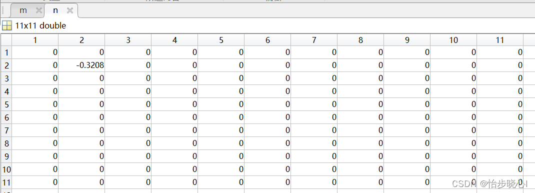
其中求解得到的n为对角矩阵,矩阵中的值为矩阵matrix_coff的特征值,m中的每一列为相应的特征值的特征向量。运行上面的代码,得到的矩阵n如下所示,由此可见方程共有11个特征值,其中-0.3208是一重特征值,0是十重特征值(好像是这么叫的):
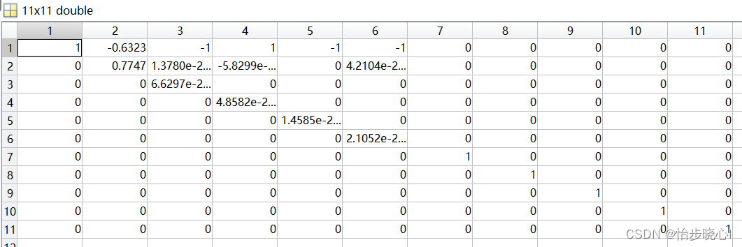
0特征值所对应的特征向量就是方程组的解,查看m矩阵,除去第2列外其余都是满足方程条件的解,其中1、3、4、5、6列没啥好看的,特征向量都差不多。但是7、8、9、10、11列非常有趣,代表sin(theta)、sin(2theta)、sin(3theta)、sin(4theta)、sin(5theta)都是方程解的一部分。这意味着对F类波形乘以1+a* sin(theta)+b* sin(2theta)+c* sin(3theta)+d* sin(4theta)+e* sin(5theta),其中a、b、c、d、e为任意值都会满足要求(但是相乘后的电压波形最小值不能小于0)。
4、恒定高效率方程的解验证
(
1
−
γ
sin
(
θ
)
)
(1 - \gamma \sin (\theta ))
(1−γsin(θ))这样的连续因子在实际使用中非常广泛,但对于更加高阶的表达式的分析较少,在此实际验证。使用CF=1-sin(theta)-sin(2theta);这样的因子与原始结果相乘,得到波形如下:

效率和对应阻抗如下所示,可以看到加上高阶的因子sin(2theta)任然不会改变波形的效率实现:

再举一个例子,使用CF=1-0.5sin(2theta);这样的因子与原始结果相乘,得到波形如下:
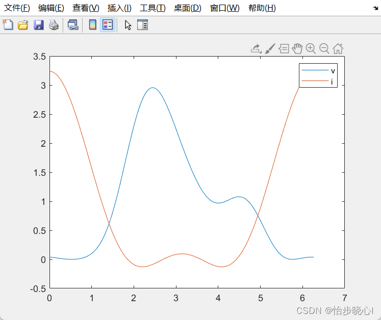
效率和对应阻抗如下所示,可以看到单独的高阶的因子sin(2theta)任然不会改变波形的效率实现:

大家可以手动试试,sin(theta)、sin(2theta)、sin(3theta)、sin(4theta)、sin(5theta)都不会改变波形的实际效率,下面给出Matlab代码:
clc
clear all
close all
theta=(0:pi/180:359.*pi/180);


% 初始化F类波形的傅里叶分量,一定要直流归一化
Vds_fouier=[1,-2/sqrt(3),0,1/(3*sqrt(3)),0,0,0,0,0,0,0];
Ids_fouier=pi*[1/pi,0.5,2/(3*pi),0,0,0,0,0,0,0,0];
% 给出连续因子的表达式
% CF=1-sin(theta)-sin(2*theta);
CF=1-0.5*sin(2*theta);
% 计算初始F类的波形
v_theta_fouier=(Vds_fouier(1)+...
    Vds_fouier(2).*cos(theta)+Vds_fouier(7).*sin(theta)+...
    Vds_fouier(3).*cos(2.*theta)+Vds_fouier(8).*sin(2.*theta)+...
    Vds_fouier(4).*cos(3.*theta)+Vds_fouier(9).*sin(3.*theta)+...
    Vds_fouier(5).*cos(4.*theta)+Vds_fouier(10).*sin(4.*theta)+...
    Vds_fouier(6).*cos(5.*theta)+Vds_fouier(11).*sin(5.*theta));
i_theta_fouier=(Ids_fouier(1)+...
    Ids_fouier(2).*cos(theta)+Ids_fouier(7).*sin(theta)+...
    Ids_fouier(3).*cos(2.*theta)+Ids_fouier(8).*sin(2.*theta)+...
    Ids_fouier(4).*cos(3.*theta)+Ids_fouier(9).*sin(3.*theta)+...
    Ids_fouier(5).*cos(4.*theta)+Ids_fouier(10).*sin(4.*theta)+...
    Ids_fouier(6).*cos(5.*theta)+Ids_fouier(11).*sin(5.*theta));
% 将初始F类的波形和连续因子相乘
v_theta_fouier_C=v_theta_fouier.*CF;

% 计算波形的傅里叶分量
Vds.dc=sum(v_theta_fouier_C)/(length(theta));
Vds.fund_cos=2*sum(v_theta_fouier_C.*cos(1*theta))/(length(theta));
Vds.fund_sin=2*sum(v_theta_fouier_C.*sin(1*theta))/(length(theta));
Vds.second_cos=2*sum(v_theta_fouier_C.*cos(2*theta))/(length(theta));
Vds.second_sin=2*sum(v_theta_fouier_C.*sin(2*theta))/(length(theta));
Vds.third_cos=2*sum(v_theta_fouier_C.*cos(3*theta))/(length(theta));
Vds.third_sin=2*sum(v_theta_fouier_C.*sin(3*theta))/(length(theta));
Vds.fourth_cos=2*sum(v_theta_fouier_C.*cos(4*theta))/(length(theta));
Vds.fourth_sin=2*sum(v_theta_fouier_C.*sin(4*theta))/(length(theta));
Vds.fifth_cos=2*sum(v_theta_fouier_C.*cos(5*theta))/(length(theta));
Vds.fifth_sin=2*sum(v_theta_fouier_C.*sin(5*theta))/(length(theta));
Ids.dc=sum(i_theta_fouier)/(length(theta));
Ids.fund_cos=2*sum(i_theta_fouier.*cos(1*theta))/(length(theta));
Ids.fund_sin=2*sum(i_theta_fouier.*sin(1*theta))/(length(theta));
Ids.second_cos=2*sum(i_theta_fouier.*cos(2*theta))/(length(theta));
Ids.second_sin=2*sum(i_theta_fouier.*sin(2*theta))/(length(theta));
Ids.third_cos=2*sum(i_theta_fouier.*cos(3*theta))/(length(theta));
Ids.third_sin=2*sum(i_theta_fouier.*sin(3*theta))/(length(theta));
Ids.fourth_cos=2*sum(i_theta_fouier.*cos(4*theta))/(length(theta));
Ids.fourth_sin=2*sum(i_theta_fouier.*sin(4*theta))/(length(theta));
Ids.fifth_cos=2*sum(i_theta_fouier.*cos(5*theta))/(length(theta));
Ids.fifth_sin=2*sum(i_theta_fouier.*sin(5*theta))/(length(theta));
Vds_fouier(1)=Vds.dc;Vds_fouier(2)=Vds.fund_cos;Vds_fouier(3)=Vds.second_cos;Vds_fouier(4)=Vds.third_cos;
Vds_fouier(5)=Vds.fourth_cos;Vds_fouier(6)=Vds.fifth_cos;Vds_fouier(7)=Vds.fund_sin;
Vds_fouier(8)=Vds.second_sin;Vds_fouier(9)=Vds.third_sin;Vds_fouier(10)=Vds.fourth_sin;Vds_fouier(11)=Vds.fifth_sin;
% 根据傅里叶分量计算阻抗和效率,归一化阻抗为Ropt
Z(1)=conj(-(Vds_fouier(2)+1j*Vds_fouier(7))/(Ids_fouier(2)+1j*Ids_fouier(7)));
Z(2)=conj(-(Vds_fouier(3)+1j*Vds_fouier(8))/(Ids_fouier(3)+1j*Ids_fouier(8)));
Z(3)=conj(-(Vds_fouier(4)+1j*Vds_fouier(9))/(Ids_fouier(4)+1j*Ids_fouier(9)));
Z(4)=conj(-(Vds_fouier(5)+1j*Vds_fouier(10))/(Ids_fouier(5)+1j*Ids_fouier(10)));
Z(5)=conj(-(Vds_fouier(6)+1j*Vds_fouier(11))/(Ids_fouier(6)+1j*Ids_fouier(11)));
Z=Z/2*pi;
disp(['Z1:',num2str(Z(1)),'   Z2:',num2str(Z(2)),'   Z3:',num2str(Z(3)),'   Z4:',num2str(Z(4)),'   Z5:',num2str(Z(5))])
P.fund=0.5*real(-(Vds.fund_cos+1j*Vds.fund_sin)*conj(Ids.fund_cos+1j*Ids.fund_sin));
P.second=0.5*real(-(Vds.second_cos+1j*Vds.second_sin)*conj(Ids.second_cos+1j*Ids.second_sin));
P.third=0.5*real(-(Vds.third_cos+1j*Vds.third_sin)*conj(Ids.third_cos+1j*Ids.third_sin));
P.fourth=0.5*real(-(Vds.fourth_cos+1j*Vds.fourth_sin)*conj(Ids.fourth_cos+1j*Ids.fourth_sin));
P.fifth=0.5*real(-(Vds.fifth_cos+1j*Vds.fifth_sin)*conj(Ids.fifth_cos+1j*Ids.fifth_sin));
disp(['P1:',num2str(P.fund),'   P2:',num2str(P.second),'   P3:',num2str(P.third),'   P4:',num2str(P.fourth),'   P5:',num2str(P.fifth)])
% 绘图
figure
plot(theta,v_theta_fouier_C);
hold on
plot(theta,i_theta_fouier);
legend('v','i')


 431
431

 被折叠的 条评论
为什么被折叠?
被折叠的 条评论
为什么被折叠?
 到【灌水乐园】发言


