


import torch
t = torch.tensor([[1,2,3],[4,5,6]])
# torch.tensor()函数将列表转换为张量
>>> print(t)
tensor([[1, 2, 3],
        [4, 5, 6]])

t1 = torch.tensor([[1,2,3],[4,5,6]],dtype = torch.float32)
可以指定元素的数据类型,这里是float32类型
>>>print(t1)
tensor([[1., 2., 3.],
        [4., 5., 6.]])

t.size() #返回张量的大小
>>> print(t.size())
torch.Size([2, 3])

t.reshape(3,2) #重新组织元素
>>> print(t.reshape(3,2))
tensor([[1, 2],
        [3, 4],
        [5, 6]])

t.dim() #返回张量的维数
>>> print(t.dim())
2

t.numel() #返回张量中元素的个数
>>> print(t.numel())
6

t.dtype #查看数据类型
>>> print(t.dtype)
torch.int64

###################################################

**构造特定大小的张量**

t1 = torch.empty() #各元素未初始化
>>>t1 = torch.empty(2)
>>> print(t1)
tensor([0.0000, 1.8750])

torch.zeros() #各元素值为0
>>> t2= torch.zeros(2)
>>> print(t2)
tensor([0., 0.])

t3 = torch.ones() #各元素为1
>>>t3 = torch.ones(2,2)
>>> print(t3)
tensor([[1., 1.],
        [1., 1.]])

torch.full() #各元素全为指定的值
>>> t4 = torch.full((2,2),3) #这里各元素全指定为3
>>> print(t4)
tensor([[3., 3.],
        [3., 3.]])

>>>t5 = torch.ones_like(t1) #构造与t1大小一样、各元素全为1的张量
>>> print(t5)
tensor([1., 1.])

############################################################
**构造等差数列和等比数列**
#首先构造等差数列,有以下三种方法:

>>> t1 = torch.arange(0,4,step=1) #构造等差数列
>>> print(t1)
tensor([0, 1, 2, 3])

>>> t2 = torch.range(0,4,step=1) #构造等差数列
>>> print(t2)
tensor([0., 1., 2., 3., 4.])

>>> t3 = torch.linspace(0,3,steps=4) #构造等差数列
>>> print(t3)
tensor([0., 1., 2., 3.])

#构造等比数列
>>> t4 = torch.logspace(0,3,steps=4)
>>> print(t4)
tensor([   1.,   10.,  100., 1000.])
#说明:torch.logspace(0,3,steps=4)中,
steps=4表示等比数列中有4个元素,
0,3表示等比数列的第一个元素和最后一个元素,
只是这里经过了以10为底的指数运算,
所以数列的第一个元素应该是10的0次方,
最后一个元素应该是10的2次方。
整据代码表示的是:
以等比数列的第一个元素为1,最后一个元素为1000,元素个数为4.

###########################################################
**构造随机张量**
torch.bernoulli(input)函数 :
input 为输入张量。
input中的每个值都在0到1之间,是概率值。
torch.bernoulli(input)函数的输出为:
大小与input张量一样的张量。
但是值全为0或1,input的值就是torch.bernoulli(input)函数取0的概率。

>>> probs = torch.full((1,10),0.7)
>>> print(probs)
tensor([[0.7000, 0.7000, 0.7000, 0.7000, 0.7000, 0.7000, 0.7000, 0.7000, 0.7000,0.7000]])
>>> print(torch.bernoulli(probs))
tensor([[1., 1., 1., 0., 1., 1., 1., 0., 1., 0.]]) #这个结果每次运行的结果不一样,因为是以概率出现的。

**torch.multinomial(input,num_samples,replacement=False)函数**
input为输入张量,
torch.multinomial(input,num_samples,replacement=False)输出的是input张量的索引
num_samples表示选取的次数;
replacement表示是否重复选取;
input的值为权重,权重越大,越可能被选中。看看下面的一个例子:
>>> weights = torch.Tensor([1, 100, 110, 50000])
>>> print(torch.multinomial(weights,4))
tensor([3, 2, 1, 0])
>>> print(torch.multinomial(weights,4))
tensor([3, 1, 2, 0])
分析:
在张量weights的4个值中,第3个值远远大于前面三个,所以它被选中的概率最大;
第1个和第2个值相差不大,所以被选中的概率相差不大;
第0个值相对最小,所以被选中的概率就最小;
所以结果基本上只会出现tensor([3, 2, 1, 0])和tensor([3, 1, 2, 0])这两种。
我们分析一下tensor([3, 2, 1, 0])这一结果。
首先,第一次被选中的是weights中的50000,它在weights中的索引为3,所以输出的第一个数是3;
依次类推,最后一个被选中的weights中的1,它在weights中的位置为0,所以输出的最后一个数是0。
语句torch.multinomial(weights,4)中的4表示选取了4次,我们来看看选取3次的情形:
>>> weights = torch.Tensor([1, 100, 110, 50000])
>>> print(torch.multinomial(weights,3))
tensor([3, 2, 1])
>>> print(torch.multinomial(weights,3))
tensor([3, 1, 2])
以上就是选取3次的结果,与选取4次是一样的道理。
我们再来看看参数replacement的作用,之前没有加入参数replacement,则默认为False;
>>> weights = torch.Tensor([1, 100, 110, 50000])
>>> print(torch.multinomial(weights,4,replacement = True))
tensor([3, 3, 3, 3])
可以看到,当参数replacement = True时,每次选择都是weights中的第3个数。

**函数torch.randperm(n)**
输入一个整数n;
输出0到n-1的一个排列。
看看下面的例子:
>>> print(torch.randperm(10))
tensor([5, 0, 2, 4, 9, 1, 6, 3, 7, 8])

**函数torch.randint(low,high,size)**
输入:下限low,上限high,输出张量的大小size
输出:生成大小为size,下限为low,上限为high的独立同均匀分布的随机整数。
看看下面的例子:
>>> print(torch.randint(2,8,(2,4)))
tensor([[2, 6, 7, 2],
        [5, 4, 5, 7]])
也可以写成
print(torch.randint(low = 2,high = 8, size = (2,4)))
tensor([[5, 5, 6, 2],
        [3, 6, 3, 2]])
注意:low和high必须为整数,否则会报错。
顺便给出一个torch.randint_like()的例子:
>>> a = torch.randint(2,8,(2,4))
>>> print(a)
tensor([[3, 4, 6, 3],
        [6, 7, 7, 3]])
>>> print(torch.randint_like(a,low = 3,high = 6))
tensor([[4, 5, 5, 3],
        [3, 3, 3, 3]])

**torch.rand(size)函数:**
输入:张量的大小size;
输出:大小为size的张量,张量中的每个值服从[0,1)之间的均匀分布
>>> t = torch.rand(2,3)
>>> print(t)
tensor([[0.6239, 0.6922, 0.9447],
        [0.4440, 0.8797, 0.4528]])
>>> print(torch.rand_like(a))
tensor([[0.2790, 0.3896, 0.0089],
        [0.7830, 0.6293, 0.0521]])

**torch.randn(size)函数**
输入:张量的大小size;
输出:大小为size的张量,张量中的每个值服从标准正态分布
>>> t = torch.randn(2,3)
>>> print(t)
tensor([[-0.0753, -0.5840, -0.7736],
        [-2.2851, -1.0012,  1.1534]])
>>> print(torch.randn_like(t))
tensor([[-0.0600,  1.0903, -0.9546],
        [-0.9317, -1.7643, -0.4342]])

**torch.normal(mean,std)函数**
输入:均值mean,和方差std;但是均值和方差都必须是张量
输出:产生的张量的值服从均值为mean,方差为std的正态分布
>>> print(torch.normal(torch.tensor([0.]),torch.tensor([1.])))
tensor([-0.1212])
>>> print(torch.normal(torch.tensor([0.,1.]),torch.tensor([1.,3.])))
tensor([0.3330, 0.8037])

**reshape()函数**
该函数只改变张量的尺寸,不改变张量元素的个数和值;
>>> t = torch.arange(12)
>>> print(t)
tensor([ 0,  1,  2,  3,  4,  5,  6,  7,  8,  9, 10, 11])
>>> t322 = t.reshape(3,2,2)
>>> print(t322)
tensor([[[ 0,  1],
         [ 2,  3]],

        [[ 4,  5],
         [ 6,  7]],

        [[ 8,  9],
         [10, 11]]])
>>> t43 = t322.reshape(4,3)
>>> print(t43)
tensor([[ 0,  1,  2],
        [ 3,  4,  5],
        [ 6,  7,  8],
        [ 9, 10, 11]])

>>> t322 = t.reshape(3,-1,2) #括号中的-1代表让函数自动计算该维度。
>>> print(t322)
tensor([[[ 0,  1],
         [ 2,  3]],

        [[ 4,  5],
         [ 6,  7]],

        [[ 8,  9],
         [10, 11]]])

**t1.squeeze()函数**
表示消除张量t1中维度为1的维度
>>> t1 = torch.arange(24).reshape(2,1,3,1,4)
>>> print(t1)
tensor([[[[[ 0,  1,  2,  3]],

          [[ 4,  5,  6,  7]],

          [[ 8,  9, 10, 11]]]],


        [[[[12, 13, 14, 15]],

          [[16, 17, 18, 19]],

          [[20, 21, 22, 23]]]]])
>>> t2 = t1.squeeze()
>>> print(t2)
tensor([[[ 0,  1,  2,  3],
         [ 4,  5,  6,  7],
         [ 8,  9, 10, 11]],

        [[12, 13, 14, 15],
         [16, 17, 18, 19],
         [20, 21, 22, 23]]])

**t.unsqueeze(dim)函数**
表示给张量t增加维度;
具体见下面例子:
>>> t = torch.arange(4) #大小为(4)
>>> print(t)
tensor([0, 1, 2, 3])
>>> print(t.unsqueeze(dim=0)) #大小为(1,4)
tensor([[0, 1, 2, 3]])
>>> print(t.unsqueeze(dim=1)) #大小为(4,1)
tensor([[0],
        [1],
        [2],
        [3]])

**t1.permute(dims)函数**
将t1的维度重新排列,但不改变t1的值
>>> t = torch.arange(4)
>>> t1 = t.reshape(2,2) #两行两列
>>> print(t1)
tensor([[0, 1],
        [2, 3]])
>>> t2 = t1.permute(dims=[1,0]) #相当于矩阵的转置。
>>> print(t2)
tensor([[0, 2],
        [1, 3]])

**t.transpose()函数和t.t()函数**
表示将张量t进行转置
>>> t = torch.tensor([[1,2],[4,6]])
>>> print(t)
tensor([[1, 2],
        [4, 6]])
>>> print(t.transpose(0,1))
tensor([[1, 4],
        [2, 6]])
>>> print(t.t())
tensor([[1, 4],
        [2, 6]])

**选取部分张量元素**
*一维张量的选取*
>>> t = torch.arange(12)
>>> print(t)
tensor([ 0,  1,  2,  3,  4,  5,  6,  7,  8,  9, 10, 11])
>>> print(t[3])
tensor(3)
>>> print(t[3:9])
tensor([3, 4, 5, 6, 7, 8])
>>> print(t[3:9:2]) #表示从第3个到第9个数之间,每隔两个数取一个
tensor([3, 5, 7])
*多维张量的选取*
>>> t = torch.arange(12).reshape(3,4)
>>> print(t)
tensor([[ 0,  1,  2,  3],
        [ 4,  5,  6,  7],
        [ 8,  9, 10, 11]])
>>> print(t[0:2,1:3])
tensor([[1, 2],
        [5, 6]])

**张量的扩展**
>>> t = torch.tensor([5,9])
>>> print(t)
tensor([5, 9])
>>> t1 = t.repeat(3,2)
>>> print(t1)
tensor([[5, 9, 5, 9],
        [5, 9, 5, 9],
        [5, 9, 5, 9]])

**张量的拼接**
>>> tp = torch.arange(12).reshape(3,4)
>>> tn = -tp
>>> tc0 = torch.cat([tp,tn],0) #此处的0代表拼接的维度
>>> tc1 = torch.cat([tp,tn],1) #此处的1代表拼接的维度
>>> print(tp)
tensor([[ 0,  1,  2,  3],
        [ 4,  5,  6,  7],
        [ 8,  9, 10, 11]])
>>> print(tn)
tensor([[  0,  -1,  -2,  -3],
        [ -4,  -5,  -6,  -7],
        [ -8,  -9, -10, -11]])
>>> print(tc0)
tensor([[  0,   1,   2,   3],
        [  4,   5,   6,   7],
        [  8,   9,  10,  11],
        [  0,  -1,  -2,  -3],
        [ -4,  -5,  -6,  -7],
        [ -8,  -9, -10, -11]])
>>> print(tc1)
tensor([[  0,   1,   2,   3,   0,  -1,  -2,  -3],
        [  4,   5,   6,   7,  -4,  -5,  -6,  -7],
        [  8,   9,  10,  11,  -8,  -9, -10, -11]])
注意:也可以拼接多个张量,我们的演示例子只给出了两个张量的拼接。

**使用torch.stack()函数进行拼接,注意它与torch.cat()函数有一定的区别**
>>> tp = torch.arange(12).reshape(3,4)
>>> tn = -tp
>>> ts0 = torch.stack([tp,tn],0)
>>> ts1 = torch.stack([tp,tn],1)
>>> print(ts0)
tensor([[[  0,   1,   2,   3],
         [  4,   5,   6,   7],
         [  8,   9,  10,  11]],

        [[  0,  -1,  -2,  -3],
         [ -4,  -5,  -6,  -7],
         [ -8,  -9, -10, -11]]])
>>> print(ts1)
tensor([[[  0,   1,   2,   3],
         [  0,  -1,  -2,  -3]],

        [[  4,   5,   6,   7],
         [ -4,  -5,  -6,  -7]],

        [[  8,   9,  10,  11],
         [ -8,  -9, -10, -11]]])
>>> print(ts0.size())
torch.Size([2, 3, 4])
>>> print(ts1.size())
torch.Size([3, 2, 4])
>>> print(ts0[0])
tensor([[ 0,  1,  2,  3],
        [ 4,  5,  6,  7],
        [ 8,  9, 10, 11]])
>>> print(ts0[1])
tensor([[  0,  -1,  -2,  -3],
        [ -4,  -5,  -6,  -7],
        [ -8,  -9, -10, -11]])

**张量的初等运算**
>>> tl = torch.tensor([[1.,2.,3.],[4.,5.,6.]])
>>> tr = torch.tensor([[7.,8.,9.],[10.,11.,12.]])
>>> print(tl + tr) #加法
tensor([[ 8., 10., 12.],
        [14., 16., 18.]])
>>> print(tl - tr) #减法
tensor([[-6., -6., -6.],
        [-6., -6., -6.]])
>>> print(tl / tr) #除法
tensor([[0.1429, 0.2500, 0.3333],
        [0.4000, 0.4545, 0.5000]])
>>> print(tl ** tr) #有理数次乘方
tensor([[1.0000e+00, 2.5600e+02, 1.9683e+04],
        [1.0486e+06, 4.8828e+07, 2.1768e+09]])
>>> print((1/tr)) #倒数
tensor([[0.1429, 0.1250, 0.1111],
        [0.1000, 0.0909, 0.0833]])
>>> print(tl ** (1/tr)) #有理数次开方
tensor([[1.0000, 1.0905, 1.1298],
        [1.1487, 1.1576, 1.1610]])

>>> t = torch.tensor([[1.,2.,3.],[4.,5.,6.]])
>>> print(t.reciprocal()) #取倒数
tensor([[1.0000, 0.5000, 0.3333],
        [0.2500, 0.2000, 0.1667]])
>>> print(t.sqrt()) #开平方
tensor([[1.0000, 1.4142, 1.7321],
        [2.0000, 2.2361, 2.4495]])
>>> print(t.rsqrt()) #先开平方,再求倒数
tensor([[1.0000, 0.7071, 0.5774],
        [0.5000, 0.4472, 0.4082]])

>>> tp = torch.pow(torch.tensor([1,2,3]),torch.tensor([2,3,4])) #幂函数
>>> print(tp)
tensor([ 1,  8, 81])

>>> torch.exp(torch.tensor([1.,2.])) #e指数函数
tensor([2.7183, 7.3891])

>>> torch.expm1(torch.tensor([1.])) #函数e^x-1
tensor([1.7183])

>>> torch.sigmoid(torch.tensor([1.])) #sigmoid函数
tensor([0.7311])

>>> torch.log(torch.tensor([1.,2.732])) #以e为底的对数
tensor([0.0000, 1.0050])

>>> torch.log2(torch.tensor([1.,2.])) #以2为底的对数
tensor([0., 1.])

>>> torch.log10(torch.tensor([1.,10.])) #以10为底的对数
tensor([0., 1.])

>>> torch.log1p(torch.tensor([0.,1.732])) 函数ln(1+x)
tensor([0.0000, 1.0050])

**三角函数:正弦、余弦、正切**
>>> torch.sin(torch.tensor([0.,3.1415926/2,3.1415926]))
tensor([0.0000e+00, 1.0000e+00, 1.5100e-07])
>>> torch.cos(torch.tensor([0.,3.1415926/2,3.1415926]))
tensor([ 1.0000e+00,  7.5498e-08, -1.0000e+00])
>>> torch.tan(torch.tensor([0.,3.1415926/4,3.1415926/2]))
tensor([0.0000e+00, 1.0000e+00, 1.3245e+07])

**反三角函数:反正弦、反余弦、反正切**
>>> torch.asin(torch.tensor([0.,1.]))
tensor([0.0000, 1.5708])
>>> torch.acos(torch.tensor([0.,1.]))
tensor([1.5708, 0.0000])
>>> torch.atan(torch.tensor([0.,1.]))
tensor([0.0000, 0.7854])

>>> torch.sign(torch.tensor([-1.1,1.2,0.])) #符号函数
tensor([-1.,  1.,  0.])

>>> torch.abs(torch.tensor([-1.1,1.2,0.])) #绝对值函数
tensor([1.1000, 1.2000, 0.0000])

>>> torch.floor(torch.tensor([-1.1,1.2,0.])) #向下取整函数
tensor([-2.,  1.,  0.])

>>> torch.ceil(torch.tensor([-1.1,1.2,0.])) #向上取整函数
tensor([-1.,  2.,  0.])

>>> torch.round(torch.tensor([-1.1,1.6,0.4])) #四舍五入函数
tensor([-1.,  2.,  0.])

>>> torch.trunc(torch.tensor([-1.1,1.6,0.4])) #去尾函数,直接去掉小数部分
tensor([-1.,  1.,  0.])

>>> torch.frac(torch.tensor([-1.9,1.6,0.4])) #取小数部分的函数
tensor([-0.9000,  0.6000,  0.4000])

**张量的部分统计函数**
>>> x = torch.rand(2,5)
>>> print(x)
tensor([[0.4610, 0.5145, 0.3761, 0.4318, 0.3433],
        [0.5433, 0.4455, 0.6578, 0.6153, 0.5263]])
>>> torch.mean(x) #求张量元素的均值
tensor(0.4915)
>>> torch.sum(x) #求张量元素的和
tensor(4.9149)
>>> torch.std(x) #标准差
tensor(0.0996)
>>> torch.var(x) #方差
tensor(0.0099)
>>> torch.prod(x) #所以元素的和
tensor(0.0007)
>>> torch.max(x) #最大值
tensor(0.6578)
>>> torch.min(x) #最小值
tensor(0.3433)
>>> torch.median(x) #中位数
tensor(0.4610)

>>> t = torch.tensor([1,2,4,5,7])
>>> print(t.kthvalue(2)) #第2大值
torch.return_types.kthvalue(
values=tensor(2),
indices=tensor(1))

>>> t = torch.tensor([3,4],dtype = torch.float32)
>>> print(t.norm(p = 1,dim = 0)) #1-范数
tensor(7.)
>>> print(t.norm(p = 2,dim = 0)) #2-范数
tensor(5.)

**比较运算**
有(<、<=、>、>=、== 和 !=)
>>> t1 = torch.tensor([1,2,4,5,7])
>>> t2 = torch.tensor([3,2,5,1,6])
>>> print(t1 > t2)
tensor([0, 0, 0, 1, 1], dtype=torch.uint8)
>>> t1 != t2
tensor([1, 0, 1, 1, 1], dtype=torch.uint8)

**逻辑运算**
torch.where()函数:
该函数有三个参数,实现的是if-else的功能。
看下面的具体例子:
>>> condition = torch.tensor([1,0,1],dtype = torch.uint8)
>>> x = torch.tensor([0.3,-0.5,0.2])
>>> y = torch.tensor([-0.2,0.5,0.3])
>>> print(torch.where(condition,x,y))
tensor([0.3000, 0.5000, 0.2000])
# condition为1的时候,选x,condition为0的时候选y。
使用蒙特卡洛算法求解圆周率pi的值
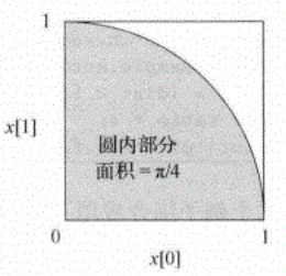
>>> def pai(sample_num):
	sample = torch.rand(sample_num,2) #产生sample_num个点
	dist = sample.norm(p=2,dim=1) #计算每个点到原点的距离
	ratio = (dist<1).float().mean() #统计小于距离小于1的均值
	pi = ratio * 4 #乘以4就是pi的值
	print(pi)
>>> pai(100000000)
tensor(3.1422)


 1万+
1万+


 被折叠的 条评论
为什么被折叠?
被折叠的 条评论
为什么被折叠?
 到【灌水乐园】发言


