扩散模型学习（一）

内容转自Unit 1: An Introduction to Diffusion Models

一、使用diffusers 库生成图片

首先安装必要的库

%pip install -qq -U diffusers datasets transformers accelerate ftfy pyarrow

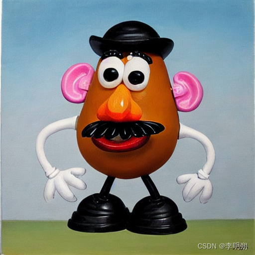
DreamBooth 是一种深度学习生成模型，用于通过微调来个性化现有的文本到图像模型。下面是一个示例

from diffusers import StableDiffusionPipeline

# Check out https://huggingface.co/sd-dreambooth-library for loads of models from the community
model_id = "sd-dreambooth-library/mr-potato-head"

# Load the pipeline
pipe = StableDiffusionPipeline.from_pretrained(model_id, torch_dtype=torch.float16).to(
    device
)

prompt = "an abstract oil painting of sks mr potato head by picasso"
image = pipe(prompt, num_inference_steps=50, guidance_scale=7.5).images[0]
image

二、训练自己的扩散模型

Diffusers 的核心 API 被分为三个主要部分:

• 管道: 从高层出发设计的多种类函数，旨在以易部署的方式，能够做到快速通过主流预训练好的扩散模型来生成样本。
• 模型: 训练新的扩散模型时用到的主流网络架构，e.g. UNet.
• 管理器 (or 调度器): 在 推理 中使用多种不同的技巧来从噪声中生成图像，同时也可以生成在 训练 中所需的带噪图像。

训练一个扩散模型的流程看起来像是这样：

1. 从训练集中加载一些图像
2. 从不同程度上加入噪声
3. 把带了不同版本噪声的数据送进模型
4. 评估模型在对这些数据做增强去噪时的表现
5. 使用这个信息来更新模型权重，然后重复此步骤

1. 下载一个训练数据集

我们会用到一个来自 Hugging Face Hub 的图像集。具体来说，是个 1000 张蝴蝶图像收藏集。也可以使用自己的数据集

import torchvision
from datasets import load_dataset
from torchvision import transforms

dataset = load_dataset("huggan/smithsonian_butterflies_subset", split="train")

# Or load images from a local folder
# dataset = load_dataset("imagefolder", data_dir="path/to/folder")

# We'll train on 32-pixel square images, but you can try larger sizes too
image_size = 32
# You can lower your batch size if you're running out of GPU memory
batch_size = 64

# Define data augmentations
preprocess = transforms.Compose(
    [
        transforms.Resize((image_size, image_size)),  # Resize
        transforms.RandomHorizontalFlip(),  # Randomly flip (data augmentation)
        transforms.ToTensor(),  # Convert to tensor (0, 1)
        transforms.Normalize([0.5], [0.5]),  # Map to (-1, 1)
    ]
)


def transform(examples):
    images = [preprocess(image.convert("RGB")) for image in examples["image"]]
    return {"images": images}


dataset.set_transform(transform)

# Create a dataloader from the dataset to serve up the transformed images in batches
train_dataloader = torch.utils.data.DataLoader(
    dataset, batch_size=batch_size, shuffle=True
)

可以从中取出一批图像数据来看一看他们是什么样子:

xb = next(iter(train_dataloader))["images"].to(device)[:8]
print("X shape:", xb.shape)
show_images(xb).resize((8 * 64, 64), resample=Image.NEAREST)

2. 定义管理器

噪声管理器决定在不同的迭代周期时分别加入多少噪声。

from diffusers import DDPMScheduler

noise_scheduler = DDPMScheduler(num_train_timesteps=1000)

示例如下：

timesteps = torch.linspace(0, 999, 8).long().to(device)
noise = torch.randn_like(xb)
noisy_xb = noise_scheduler.add_noise(xb, noise, timesteps)
print("Noisy X shape", noisy_xb.shape)
show_images(noisy_xb).resize((8 * 64, 64), resample=Image.NEAREST)

3.定义模型

大多数扩散模型使用的模型结构都是一些 U-net 的变形。Diffusers 为我们提供了一个易用的UNet2DModel类，用来在 PyTorch 创建所需要的结构。

from diffusers import UNet2DModel

# Create a model
model = UNet2DModel(
    sample_size=image_size,  # the target image resolution
    in_channels=3,  # the number of input channels, 3 for RGB images
    out_channels=3,  # the number of output channels
    layers_per_block=2,  # how many ResNet layers to use per UNet block
    block_out_channels=(64, 128, 128, 256),  # More channels -> more parameters
    down_block_types=(
        "DownBlock2D",  # a regular ResNet downsampling block
        "DownBlock2D",
        "AttnDownBlock2D",  # a ResNet downsampling block with spatial self-attention
        "AttnDownBlock2D",
    ),
    up_block_types=(
        "AttnUpBlock2D",
        "AttnUpBlock2D",  # a ResNet upsampling block with spatial self-attention
        "UpBlock2D",
        "UpBlock2D",  # a regular ResNet upsampling block
    ),
)
model.to(device);

4.开始训练

对于每一批的数据的训练过程包括

1. 随机取样几个迭代周期
2. 根据预设为数据加入噪声
3. 把带噪数据送入模型
4. 使用 MSE 作为损失函数来比较目标结果与模型预测结果（在这里是加入噪声的场景）
5. 通过loss.backward ()与optimizer.step ()来更新模型参数

# Set the noise scheduler
noise_scheduler = DDPMScheduler(
    num_train_timesteps=1000, beta_schedule="squaredcos_cap_v2"
)

# Training loop
optimizer = torch.optim.AdamW(model.parameters(), lr=4e-4)

losses = []

for epoch in range(30):
    for step, batch in enumerate(train_dataloader):
        clean_images = batch["images"].to(device)
        # Sample noise to add to the images
        noise = torch.randn(clean_images.shape).to(clean_images.device)
        bs = clean_images.shape[0]

        # Sample a random timestep for each image
        timesteps = torch.randint(
            0, noise_scheduler.num_train_timesteps, (bs,), device=clean_images.device
        ).long()

        # Add noise to the clean images according to the noise magnitude at each timestep
        noisy_images = noise_scheduler.add_noise(clean_images, noise, timesteps)

        # Get the model prediction
        noise_pred = model(noisy_images, timesteps, return_dict=False)[0]

        # Calculate the loss
        loss = F.mse_loss(noise_pred, noise)
        loss.backward(loss)
        losses.append(loss.item())

        # Update the model parameters with the optimizer
        optimizer.step()
        optimizer.zero_grad()

    if (epoch + 1) % 5 == 0:
        loss_last_epoch = sum(losses[-len(train_dataloader) :]) / len(train_dataloader)
        print(f"Epoch:{epoch+1}, loss: {loss_last_epoch}")

5.使用训练好的模型

使用训练好的模型简历管线

from diffusers import DDPMPipeline

image_pipe = DDPMPipeline(unet=model, scheduler=noise_scheduler)
pipeline_output = image_pipe()
pipeline_output.images[0]

保存至本地

image_pipe.save_pretrained("my_pipeline")

三、从零开始训练扩散模型

在不使用diffusers库的情况下从零开始训练一个扩散模型

1.数据准备

这里使用MINST数据集

dataset = torchvision.datasets.MNIST(root="mnist/", train=True, download=True, transform=torchvision.transforms.ToTensor())
train_dataloader = DataLoader(dataset, batch_size=8, shuffle=True)

查看图片

x, y = next(iter(train_dataloader))
print('Input shape:', x.shape)
print('Labels:', y)
plt.imshow(torchvision.utils.make_grid(x)[0], cmap='Greys');

2.损坏过程（添加噪声）

def corrupt(x, amount):
  """Corrupt the input `x` by mixing it with noise according to `amount`"""
  noise = torch.rand_like(x)
  amount = amount.view(-1, 1, 1, 1) # Sort shape so broadcasting works
  return x*(1-amount) + noise*amount 

可视化该过程

# Plotting the input data
fig, axs = plt.subplots(2, 1, figsize=(12, 5))
axs[0].set_title('Input data')
axs[0].imshow(torchvision.utils.make_grid(x)[0], cmap='Greys')

# Adding noise
amount = torch.linspace(0, 1, x.shape[0]) # Left to right -> more corruption
noised_x = corrupt(x, amount)

# Plottinf the noised version
axs[1].set_title('Corrupted data (-- amount increases -->)')
axs[1].imshow(torchvision.utils.make_grid(noised_x)[0], cmap='Greys');

3.模型

简单的Unet模型示例

class BasicUNet(nn.Module):
    """A minimal UNet implementation."""
    def __init__(self, in_channels=1, out_channels=1):
        super().__init__()
        self.down_layers = torch.nn.ModuleList([ 
            nn.Conv2d(in_channels, 32, kernel_size=5, padding=2),
            nn.Conv2d(32, 64, kernel_size=5, padding=2),
            nn.Conv2d(64, 64, kernel_size=5, padding=2),
        ])
        self.up_layers = torch.nn.ModuleList([
            nn.Conv2d(64, 64, kernel_size=5, padding=2),
            nn.Conv2d(64, 32, kernel_size=5, padding=2),
            nn.Conv2d(32, out_channels, kernel_size=5, padding=2), 
        ])
        self.act = nn.SiLU() # The activation function
        self.downscale = nn.MaxPool2d(2)
        self.upscale = nn.Upsample(scale_factor=2)

    def forward(self, x):
        h = []
        for i, l in enumerate(self.down_layers):
            x = self.act(l(x)) # Through the layer and the activation function
            if i < 2: # For all but the third (final) down layer:
              h.append(x) # Storing output for skip connection
              x = self.downscale(x) # Downscale ready for the next layer
              
        for i, l in enumerate(self.up_layers):
            if i > 0: # For all except the first up layer
              x = self.upscale(x) # Upscale
              x += h.pop() # Fetching stored output (skip connection)
            x = self.act(l(x)) # Through the layer and the activation function
            
        return x

4. 训练模型

训练模型的步骤：

1. 获取一批数据
2. 添加随机噪声
3. 将数据输入模型
4. 将模型预测与干净图像进行比较，以计算loss
5. 更新模型的参数。

# Dataloader (you can mess with batch size)
batch_size = 128
train_dataloader = DataLoader(dataset, batch_size=batch_size, shuffle=True)

# How many runs through the data should we do?
n_epochs = 3

# Create the network
net = BasicUNet()
net.to(device)

# Our loss finction
loss_fn = nn.MSELoss()

# The optimizer
opt = torch.optim.Adam(net.parameters(), lr=1e-3) 

# Keeping a record of the losses for later viewing
losses = []

# The training loop
for epoch in range(n_epochs):

    for x, y in train_dataloader:

        # Get some data and prepare the corrupted version
        x = x.to(device) # Data on the GPU
        noise_amount = torch.rand(x.shape[0]).to(device) # Pick random noise amounts
        noisy_x = corrupt(x, noise_amount) # Create our noisy x

        # Get the model prediction
        pred = net(noisy_x)

        # Calculate the loss
        loss = loss_fn(pred, x) # How close is the output to the true 'clean' x?

        # Backprop and update the params:
        opt.zero_grad()
        loss.backward()
        opt.step()

        # Store the loss for later
        losses.append(loss.item())

    # Print our the average of the loss values for this epoch:
    avg_loss = sum(losses[-len(train_dataloader):])/len(train_dataloader)
    print(f'Finished epoch {epoch}. Average loss for this epoch: {avg_loss:05f}')

# View the loss curve
plt.plot(losses)
plt.ylim(0, 0.1);

5.生成图像（采样方法）

下面是给定噪声输入生成图像的方法，当噪声水平非常高时，模型能够获得的信息就开始逐渐减少。

#@markdown Visualizing model predictions on noisy inputs:

# Fetch some data
x, y = next(iter(train_dataloader))
x = x[:8] # Only using the first 8 for easy plotting

# Corrupt with a range of amounts
amount = torch.linspace(0, 1, x.shape[0]) # Left to right -> more corruption
noised_x = corrupt(x, amount)

# Get the model predictions
with torch.no_grad():
  preds = net(noised_x.to(device)).detach().cpu()

# Plot
fig, axs = plt.subplots(3, 1, figsize=(12, 7))
axs[0].set_title('Input data')
axs[0].imshow(torchvision.utils.make_grid(x)[0].clip(0, 1), cmap='Greys')
axs[1].set_title('Corrupted data')
axs[1].imshow(torchvision.utils.make_grid(noised_x)[0].clip(0, 1), cmap='Greys')
axs[2].set_title('Network Predictions')
axs[2].imshow(torchvision.utils.make_grid(preds)[0].clip(0, 1), cmap='Greys');

因此，我们使用采样的方法

#@markdown Sampling strategy: Break the process into 5 steps and move 1/5'th of the way there each time:
#@markdown Showing more results, using 40 sampling steps
n_steps = 40
x = torch.rand(64, 1, 28, 28).to(device)
for i in range(n_steps):
  noise_amount = torch.ones((x.shape[0], )).to(device) * (1-(i/n_steps)) # Starting high going low
  with torch.no_grad():
    pred = net(x)
  mix_factor = 1/(n_steps - i)
  x = x*(1-mix_factor) + pred*mix_factor
fig, ax = plt.subplots(1, 1, figsize=(12, 12))
ax.imshow(torchvision.utils.make_grid(x.detach().cpu(), nrow=8)[0].clip(0, 1), cmap='Greys')