R实战 | 环状热图(circos)

circular_heatmap

「之前画过的热图：」

1. 跟着 Cell 学作图 | 复杂热图(ComplexHeatmap)

2. 跟着 Nature 学作图 | 复杂热图2.0(连续+分类变量)

3. R实战 | 复杂热图3.0(ComplexHeatmap)

本期图片

❝

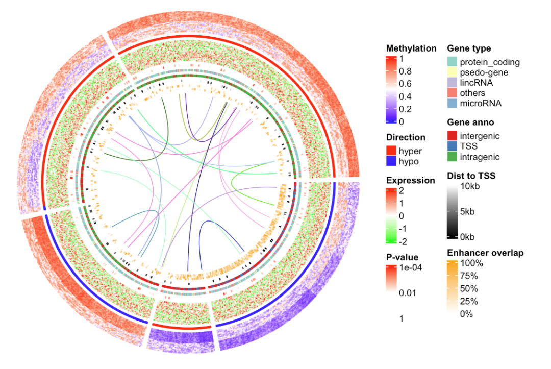
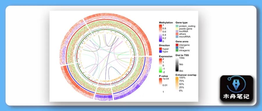
将上一期的热图掰弯，并随机给differetially methylated regions (DMRs)加个几个相互作用。

❞

示例数据和代码领取

点赞、在看 本文，分享至朋友圈集赞20个并保留30分钟，截图发至微信mzbj0002领取。

「木舟笔记2022年度VIP可免费领取」。

木舟笔记2022年度VIP企划

「权益：」

1. 「2022」年度木舟笔记所有推文示例数据及代码(「在VIP群里实时更新」)。

   
   data+code

2. 木舟笔记「科研交流群」。

3. 「半价」购买跟着Cell学作图系列合集(免费教程+代码领取)|跟着Cell学作图系列合集。

「收费：」

「99￥/人」。可添加微信：mzbj0002 转账，或直接在文末打赏。

绘制

示例数据

rm(list = ls())
# devtools::install_github("jokergoo/Complexheatmap")
library(ComplexHeatmap)
library(circlize)
library(RColorBrewer)
# 载入示例数据
res_list = readRDS("meth.rds")
str(res_list)
type = res_list$type
mat_meth = res_list$mat_meth
mat_expr = res_list$mat_expr
direction = res_list$direction
cor_pvalue = res_list$cor_pvalue
gene_type = res_list$gene_type
anno_gene = res_list$anno_gene
dist = res_list$dist
anno_enhancer = res_list$anno_enhancer


source("random_matrices.R")

绘制

set.seed(123)
km = kmeans(mat_meth, centers = 5)$cluster
# 一圈一圈轨迹叠加

col_meth = colorRamp2(c(0, 0.5, 1), c("blue", "white", "red"))
circos.heatmap(mat_meth, split = km, col = col_meth, track.height = 0.12)

col_direction = c("hyper" = "red", "hypo" = "blue")
circos.heatmap(direction, col = col_direction, track.height = 0.01)

col_expr = colorRamp2(c(-2, 0, 2), c("green", "white", "red"))
circos.heatmap(mat_expr, col = col_expr, track.height = 0.12)

col_pvalue = colorRamp2(c(0, 2, 4), c("white", "white", "red"))
circos.heatmap(cor_pvalue, col = col_pvalue, track.height = 0.01)

col_gene_type = structure(brewer.pal(length(unique(gene_type)), "Set3"), names = unique(gene_type))
circos.heatmap(gene_type, col = col_gene_type, track.height = 0.01)

col_anno_gene = structure(brewer.pal(length(unique(anno_gene)), "Set1"), names = unique(anno_gene))
circos.heatmap(anno_gene, col = col_anno_gene, track.height = 0.01) 

col_dist = colorRamp2(c(0, 10000), c("black", "white"))
circos.heatmap(dist, col = col_dist, track.height = 0.01)

col_enhancer = colorRamp2(c(0, 1), c("white", "orange"))
circos.heatmap(anno_enhancer, col = col_enhancer, track.height = 0.03)

circos.clear()

df_link = data.frame(
  from_index = sample(nrow(mat_meth), 20),
  to_index = sample(nrow(mat_meth), 20)
)


circlize_plot = function() {
  circos.heatmap(mat_meth, split = km, col = col_meth, track.height = 0.12)
  circos.heatmap(direction, col = col_direction, track.height = 0.01)
  circos.heatmap(mat_expr, col = col_expr, track.height = 0.12)
  circos.heatmap(cor_pvalue, col = col_pvalue, track.height = 0.01)
  circos.heatmap(gene_type, col = col_gene_type, track.height = 0.01)
  circos.heatmap(anno_gene, col = col_anno_gene, track.height = 0.01) 
  circos.heatmap(dist, col = col_dist, track.height = 0.01)
  circos.heatmap(anno_enhancer, col = col_enhancer, track.height = 0.03)
  
  for(i in seq_len(nrow(df_link))) {
    circos.heatmap.link(df_link$from_index[i],
                        df_link$to_index[i],
                        col = rand_color(1))
  }
  circos.clear()
}

lgd_meth = Legend(title = "Methylation", col_fun = col_meth)
lgd_direction = Legend(title = "Direction", at = names(col_direction), 
                       legend_gp = gpar(fill = col_direction))
lgd_expr = Legend(title = "Expression", col_fun = col_expr)
lgd_pvalue = Legend(title = "P-value", col_fun = col_pvalue, at = c(0, 2, 4), 
                    labels = c(1, 0.01, 0.0001))
lgd_gene_type = Legend(title = "Gene type", at = names(col_gene_type), 
                       legend_gp = gpar(fill = col_gene_type))
lgd_anno_gene = Legend(title = "Gene anno", at = names(col_anno_gene), 
                       legend_gp = gpar(fill = col_anno_gene))
lgd_dist = Legend(title = "Dist to TSS", col_fun = col_dist, 
                  at = c(0, 5000, 10000), labels = c("0kb", "5kb", "10kb"))
lgd_enhancer = Legend(title = "Enhancer overlap", col_fun = col_enhancer, 
                      at = c(0, 0.25, 0.5, 0.75, 1), labels = c("0%", "25%", "50%", "75%", "100%"))
library(gridBase)
plot.new()
circle_size = unit(1, "snpc") # snpc unit gives you a square region

pushViewport(viewport(x = 0, y = 0.5, width = circle_size, height = circle_size,
                      just = c("left", "center")))
par(omi = gridOMI(), new = TRUE)
circlize_plot()
upViewport()

h = dev.size()[2]
lgd_list = packLegend(lgd_meth, lgd_direction, lgd_expr, lgd_pvalue, lgd_gene_type, 
                      lgd_anno_gene, lgd_dist, lgd_enhancer, max_height = unit(0.9*h, "inch"))
draw(lgd_list, x = circle_size, just = "left")

result

参考

1. Supplementary S3. Correlations between methylation, expression and other genomic features (jokergoo.github.io)

2. Chapter 6 The circos.heatmap() function | Circular Visualization in R (jokergoo.github.io)

往期

1. CNS图表复现|生信分析|R绘图 资源分享&讨论群！

2. 这图怎么画| 有点复杂的散点图

3. 这图怎么画 | 相关分析棒棒糖图

4. 组学生信| Front Immunol |基于血清蛋白质组早期诊断标志筛选的简单套路

5. (免费教程+代码领取)|跟着Cell学作图系列合集

6. Q&A | 如何在论文中画出漂亮的插图？

7. 跟着 Cell 学作图 | 桑葚图(ggalluvial)

8. R实战 | Lasso回归模型建立及变量筛选

9. 跟着 NC 学作图 | 互作网络图进阶(蛋白+富集通路)(Cytoscape)

10. R实战 | 给聚类加个圈圈(ggunchull)

11. R实战 | NGS数据时间序列分析(maSigPro)

12. 跟着 Cell 学作图 | 韦恩图(ggVennDiagram)

---

木舟笔记矩阵