◇【论文_20180226v1_20181022v3】Addressing Function Approximation Error in Actor-Critic Methods 【 TD3 】

https://arxiv.org/abs/1802.09477

Addressing Function Approximation Error in Actor-Critic Methods

加拿大 麦吉尔大学 ICML 2018

摘要

In value-based reinforcement learning methods such as deep Q-learning, function approximation errors are known to lead to overestimated value estimates and suboptimal policies. 【在…方法中，存在…问题】
在基于价值的强化学习方法中，如 deep Q-learning，已知函数近似误差会导致高估的价值估计以及次优策略。
We show that this problem persists in an actor-critic setting and propose novel mechanisms to minimize its effects on both the actor and the critic. 【提出新的机制 来缓解该问题】
我们证实这个问题在 actor-critic 设置中仍然存在，并提出了新的机制来尽可能减少其对 actor 和 critic 的影响。
Our algorithm builds on Double Q-learning, by taking the minimum value between a pair of critics to limit overestimation. 【算法的关键 idea】
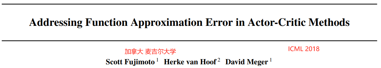
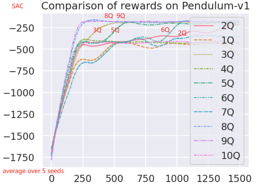
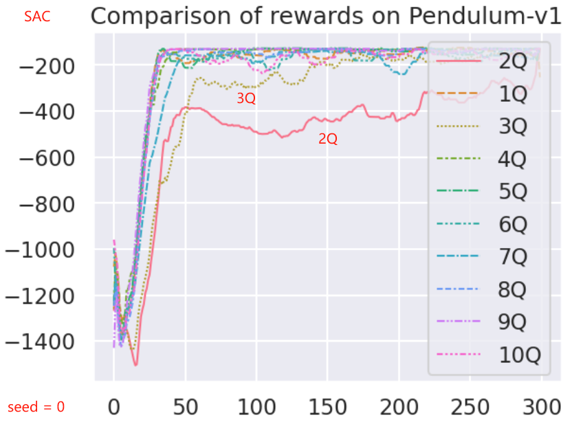
我们的算法基于 Double Q-learning，通过在一对 critics 之间取最小值来限制高估。【要是更多 critics 之间取最小值，会提升效果吗 】

• ——> 〔 从段后补充的实验，可以看到有提升的可能性很大，但也要注意 10Q 的多种子平均时的奖励并不是最高的。说明 10Q 时某些种子情形下是性能降低的 〕

We draw the connection between target networks and overestimation bias, and suggest delaying policy updates to reduce per-update error and further improve performance.
我们绘制了目标网络与高估偏差之间的联系，并建议延迟策略更新以减小每次更新误差并进一步提高性能。
We evaluate our method on the suite of OpenAI gym tasks, outperforming the state of the art in every environment tested. 【在哪些任务上进行了评估，SOTA】
我们在 OpenAI gym 任务套件中评估了我们的方法，在每个测试环境中都优于最先进的方法。

critic 和 目标 critic 的对数对训练的影响

1. 引言

In reinforcement learning problems with discrete action spaces, the issue of value overestimation as a result of function approximation errors is well-studied.
在具有离散动作空间的强化学习问题中，由于 函数近似误差 导致的 价值高估问题得到了充分的研究。
However, similar issues with actor-critic methods in continuous control domains have been largely left untouched.
然而，在连续控制域中，与 actor-critic 方法类似的问题基本上没有被触及。
In this paper, we show overestimation bias and the accumulation of error in temporal difference methods are present in an actor-critic setting.
在本文中，我们证实了高估偏差和 时序差分方法中的误差积累存在于 actor-critic 设置中。
Our proposed method addresses these issues, and greatly outperforms the current state of the art.
我们提出的方法解决了这些问题，并且大大优于当前的最先进技术水平。

Overestimation bias is a property of Q-learning in which the maximization of a noisy value estimate induces a consistent overestimation (Thrun & Schwartz, 1993).
高估偏差是 Q-learning 的一个特性，其中带噪声的价值估计的最大化会导致一致的过高估计 (Thrun & Schwartz, 1993)。
In a function approximation setting, this noise is unavoidable given the imprecision of the estimator.
在函数近似设置中，由于估计器的不精确，这种噪声是不可避免的。
This inaccuracy is further exaggerated by the nature of temporal difference learning (Sutton, 1988), in which an estimate of the value function is updated using the estimate of a subsequent state.
时序差分学习的本质进一步夸大了这种不准确性(Sutton, 1988)，其使用后续状态的估计来更新价值函数的估计。
This means using an imprecise estimate within each update will lead to an accumulation of error.
这意味着在每次更新中使用不精确的估计将导致误差的累积。
Due to overestimation bias, this accumulated error can cause arbitrarily bad states to be estimated as high value, resulting in suboptimal policy updates and divergent behavior.
由于高估偏差，这种累积误差可能导致任意不良状态被估计为高值，从而导致次优策略更新和不同的行为。

This paper begins by establishing this overestimation property is also present for deterministic policy gradients (Silver et al., 2014), in the continuous control setting.
本文首先建立了这种高估特性也存在于连续控制设置中的确定性策略梯度中(Silver et al.， 2014)。
Furthermore, we find the ubiquitous solution in the discrete action setting, Double DQN (Van Hasselt et al., 2016), to be ineffective in an actor-critic setting.
此外，我们发现 在离散动作设置中普遍存在的解决方案 Double DQN (Van Hasselt et al.， 2016) 在 actor-critic 设置中是无效的 。
During training, Double DQN estimates the value of the current policy with a separate target value function, allowing actions to be evaluated without maximization bias.
在训练期间，Double DQN 使用单独的目标价值函数估计当前策略的值，允许在没有最大化偏差的情况下评估动作。
Unfortunately, due to the slow-changing policy in an actor-critic setting, the current and target value estimates remain too similar to avoid maximization bias.
不幸的是，由于 actor-critic 设置中缓慢变化的策略，当前和目标价值估计仍然过于相似，无法避免最大化偏差。
This can be dealt with by adapting an older variant, Double Q-learning (Van Hasselt, 2010), to an actor-critic format by using a pair of independently trained critics.
这可以通过使用一对独立训练的 critics，将较早的变体 Double Q-learning (Van Hasselt, 2010) 调整为 actor-critic 格式来解决。
While this allows for a less biased value estimation, even an unbiased estimate with high variance can still lead to future overestimations in local regions of state space, which in turn can negatively affect the global policy.
虽然这允许偏差较小的价值估计，但即使是具有高方差的无偏估计也可能导致在状态空间局部区域的未来高估，这反过来可能对全局策略产生负面影响。
To address this concern, we propose a clipped Double Q-learning variant which leverages the notion that a value estimate suffering from overestimation bias can be used as an approximate upper-bound to the true value estimate.
为了解决这个问题，我们提出了一个裁剪的 Double Q-learning 变体，它利用了这样一个概念，即遭受高估偏差的价值估计可以用作真实价值估计的近似上界。
This favors underestimations, which do not tend to be propagated during learning, as actions with low value estimates are avoided by the policy.
这有利于低估，在学习过程中不倾向于传播，因为策略避开了具有低价值估计的动作。

Given the connection of noise to overestimation bias, this paper contains a number of components that address variance reduction.
考虑到噪声与高估偏差的联系，本文包含了一些解决方差减少的组件。
First, we show that target networks, a common approach in deep Q-learning methods, are critical for variance reduction by reducing the accumulation of errors.
首先，我们证实目标网络 (deep Q-learning 方法中的一种常见方法) 对于通过减少误差积累来减小方差至关重要。
Second, to address the coupling of value and policy, we propose delaying policy updates until the value estimate has converged.
其次，为了解决价值和策略的耦合问题，我们建议延迟策略更新，直到价值估计收敛。
Finally, we introduce a novel regularization strategy, where a SARSA-style update bootstraps similar action estimates to further reduce variance.
最后，我们引入了一种新的正则化策略，其中 SARSA 风格的更新 自举类似的动作估计以进一步减小方差。

Our modifications are applied to the state of the art actor-critic method for continuous control, Deep Deterministic Policy Gradient algorithm (DDPG) (Lillicrap et al., 2015), to form the Twin Delayed Deep Deterministic policy gradient algorithm (TD3), an actor-critic algorithm which considers the interplay between function approximation error in both policy and value updates.
我们的修改应用于连续控制中最先进的 actor-critic 方法，深度确定性策略梯度算法 (DDPG) (Lillicrap等人，2015)，形成了双延迟深度确定性策略梯度算法 (TD3)，这是一种 actor-critic 算法，它考虑了策略和价值更新中函数近似误差之间的相互影响。
We evaluate our algorithm on seven continuous control domains from OpenAI gym (Brockman et al., 2016), where we outperform the state of the art by a wide margin.
我们在 OpenAI gym 的七个连续控制域 (Brockman et al.， 2016)上评估了我们的算法，在这些控制域上，我们的表现远远超过了最先进的技术。

Given the recent concerns in reproducibility (Henderson et al., 2017), we run our experiments across a large number of seeds with fair evaluation metrics, perform ablation studies across each contribution, and open source both our code and learning curves (https://github.com/sfujim/TD3).
考虑到最近对可重复性的担忧 (Henderson 等人，2017)，我们在大量具有公平评估指标的种子上运行实验，对每个贡献进行消融研究，并开源我们的代码和学习曲线(https://github.com/sfujim/TD3)。

2. 相关工作

Function approximation error and its effect on bias and variance in reinforcement learning algorithms have been studied in prior works (Pendrith et al., 1997; Mannor et al., 2007).
函数近似误差及其对强化学习算法中的偏差和方差的影响已经在先前的工作中进行了研究。
Our work focuses on two outcomes that occur as the result of estimation error, namely overestimation bias and a high variance build-up.
我们的工作重点是由于估计误差而产生的两种结果，即高估偏差和高方差累积。

Several approaches exist to reduce the effects of overestimation bias due to function approximation and policy optimization in Q-learning.
在 Q-learning 中，由于函数近似和策略优化，有几种方法可以减少高估偏差的影响。
Double Q-learning uses two independent estimators to make unbiased value estimates (Van Hasselt, 2010; Van Hasselt et al., 2016).
Double Q-learning 使用两个独立的估计器进行无偏价值估计。
Other approaches have focused directly on reducing the variance (Anschel et al., 2017), minimizing over-fitting to early high variance estimates (Fox et al., 2016), or through corrective terms (Lee et al., 2013).
其他方法直接侧重于减小方差 (Anschel等人，2017)，最小化对早期高方差估计的过拟合 (Fox 等人，2016)，或通过校正项(Lee等人，2013)。
Further, the variance of the value estimate has been considered directly for risk-aversion (Mannor & Tsitsiklis, 2011) and exploration (O’Donoghue et al., 2017), but without connection to overestimation bias.
此外，价值估计的方差已被直接用于风险规避 (Mannor & Tsitsiklis, 2011) 和探索(O’Donoghue et al.， 2017)，但与高估偏差无关。

The concern of variance due to the accumulation of error in temporal difference learning has been largely dealt with by either minimizing the size of errors at each time step or mixing off-policy and Monte-Carlo returns.
在时序差分学习中，由于误差累积而引起的方差问题主要通过最小化每个时间步的误差大小或混合异策略的off-policy 和 蒙特卡罗回报 来解决。
Our work shows the importance of a standard technique, target networks, for the reduction of per-update error, and develops a regularization technique for the variance reduction by averaging over value estimates.
我们的工作证实了标准技术，目标网络，对于减小每次更新误差的重要性，并开发了一种正则化技术，通过对价值估计进行平均来减少方差。
Concurrently, Nachum et al. (2018) showed smoothed value functions could be used to train stochastic policies with reduced variance and improved performance.
同时，Nachum 等人(2018) 表明，平滑的价值函数可以用来训练方差减小、性能提高的随机策略。
Methods with multi-step returns offer a trade-off between accumulated estimation bias and variance induced by the policy and the environment.
多步回报 的方法提供了 累积估计偏差 和 由策略和环境引起的方差之间的权衡。
These methods have been shown to be an effective approach, through importance sampling (Precup et al., 2001; Munos et al., 2016), distributed methods (Mnih et al., 2016; Espeholt et al., 2018), and approximate bounds (He et al., 2016).
通过重要性采样，分布式方法 和 近似边界，这些方法已被证明是一种有效的方法。
However, rather than provide a direct solution to the accumulation of error, these methods circumvent the problem by considering a longer horizon.
然而，这些方法并没有直接解决误差积累的问题，而是通过考虑更长的视界来规避问题。
Another approach is a reduction in the discount factor (Petrik & Scherrer, 2009), reducing the contribution of each error.
另一种方法是减小折扣因子(Petrik & Scherrer, 2009)，减小每个误差的贡献。

Our method builds on the Deterministic Policy Gradient algorithm (DPG) (Silver et al., 2014), an actor-critic method which uses a learned value estimate to train a deterministic policy.
我们的方法基于 确定性策略梯度算法 (DPG) (Silver 等人，2014)，一种使用习得的价值估计来训练确定性策略的 actor-critic 方法。
An extension of DPG to deep reinforcement learning, DDPG (Lillicrap et al., 2015), has shown to produce state of the art results with an efficient number of iterations.
将 DPG 扩展到深度强化学习的 DDPG (Lillicrap 等人，2015) 已经证明可以通过高效的多次迭代产生最先进的结果。
Orthogonal to our approach, recent improvements to DDPG include distributed methods (Popov et al., 2017), along with multi-step returns and prioritized experience replay (Schaul et al., 2016; Horgan et al., 2018), and distributional methods (Bellemare et al., 2017; Barth-Maron et al., 2018).
与我们的方法正交，DDPG 的最新改进包括分布式方法 (Popov等人，2017)，以及多步回报和优先经验回放 (Schaul等人，2016;Horgan 等人，2018)和 分配方法 (Bellemare 等人，2017;Barth-Maron et al.， 2018)。

3. 背景

强化学习考虑了代理agent 与其环境相互作用的范式，目的是学习最大化奖励reward 的行为。
在每个离散时间步 $t$，在给定 state状态 $s\in \mathcal{S}$ 下，agent 根据policy策略 $\pi :\mathcal{S}\to \mathcal{A}$ 选择action动作 $a\in \mathcal{A}$，接收奖励 $r$ 和环境的新状态 $s^{\prime }$。
回报return 定义为奖励的折扣总和 $R_t=\sum _{i=t}^T{\gamma }^{i-t}r(s_i,a_i)$，其中 $\gamma$ 是决定短期奖励优先级的折扣因子。

在强化学习中，目标是找到参数为 $\varphi$ 的最优策略 ${\pi }_{\varphi }$，最大化回报的期望 $J(\varphi )={\mathbb{E}}_{s_i\sim p_{\pi },a_i\sim \pi }[R_0]$。
对于连续控制，参数化策略 ${\pi }_{\varphi }$ 可以通过取回报的期望的梯度 ${\nabla }_{\varphi }J(\varphi )$ 来更新。
在 actor-critic 方法中，被称为 actor 的策略可以通过确定性策略梯度算法进行更新 (Silver et al.， 2014):
  ~  
${\nabla }_{\varphi }J(\varphi )={\mathbb{E}}_{s\sim p_{\pi }}[{\nabla }_a{Q}^{\pi }(s,a){|}_{a=\pi (s)}{\nabla }_{\varphi }{\pi }_{\varphi }(s)](1)$
  ~  
$Q^{\pi }(s,a)={\mathbb{E}}_{s_i\sim p_{\pi },a_i\sim \pi }[R_t|s,a]$：在状态 $s$ 下执行动作 $a$ 并在其后遵循 $\pi$ 的回报的期望 称为 critic 或 价值函数。

在 Q-learning 中，可以使用 时序差分学习 来学习价值函数 (Sutton, 1988;Watkins, 1989)，一个基于 Bellman 公式 的更新规则(Bellman, 1957)。
Bellman 公式是 状态-动作对 $(s,a)$ 的价值 与 后续状态-动作对 $(s^{\prime },a^{\prime })$ 的价值之间的基本关系:
  ~  
$Q^{\pi }(s,a)=r+\gamma {\mathbb{E}}_{s^{\prime },a^{\prime }}[Q^{\pi }(s^{\prime },a^{\prime })],a^{\prime }\sim \pi (s^{\prime })(2)$
  ~  
对于大的状态空间，可以使用参数为 $\theta$ 的可微函数近似器 $Q_{\theta }(s,a)$ 估计价值。
在 deep Q-learning (Mnih et al.， 2015) 中，网络通过使用时序差分学习更新，并使用二次冻结目标网络 $Q_{{\theta }^{\prime }}(s,a)$ 在多个更新内保持固定的目标 $y$：
  ~  
$y=r+\gamma Q_{{\theta }^{\prime }}(s^{\prime },a^{\prime })a^{\prime }\sim {\pi }_{{\varphi }^{\prime }}(s^{\prime })(3)$
  ~  
其中动作是从目标 actor 网络 ${\pi }_{{\varphi }^{\prime }}$ 中选择的。
目标网络的权重要么定期更新以精确匹配当前网络的权重，要么在每个时间步按一定比例 $\tau$ 更新 ${\theta }^{\prime }\leftarrow \tau \theta +(1-\tau ){\theta }^{\prime }$ 。〔 $\tau \ll 1$， 每个时间步更新很小的部分 〕
这种更新可以以异策略 off-policy 方式应用，从经验回放缓冲区中随机取样小批量的转换transitions (Lin, 1992)。

4. 高估偏差

对于离散动作的 Q-learning，用贪心目标 $y=r+\gamma {\max }_{a^{\prime }}Q(s^{\prime },a^{\prime })$ 更新价值估计，然而，如果目标易受到误差 $ϵ$ 的影响，那么该价值的最大值随着误差通常会大于真实最大值 ${\mathbb{E}}_{ϵ}[{\max }_{a^{\prime }}(Q(s^{\prime },a^{\prime })+ϵ)]\ge {\max }_{a^{\prime }}Q(s^{\prime },a^{\prime })$ (Thrun & Schwartz, 1993)。
As a result, even initially zero-mean error can cause value updates to result in a consistent overestimation bias, which is then propagated through the Bellman equation.
因此，即使最初的零均值误差会导致 得到一致的高估偏差 的价值更新 ，然后通过 Bellman 公式传播。
This is problematic as errors induced by function approximation are unavoidable.
这是有问题的，因为由函数近似引起的误差是不可避免的。

While in the discrete action setting overestimation bias is an obvious artifact from the analytical maximization, the presence and effects of overestimation bias is less clear in an actor-critic setting where the policy is updated via gradient descent.
虽然在离散动作设置中，高估偏差是分析最大化的明显产物，但在通过梯度下降更新策略的 actor-critic 设置中，高估偏差的存在和影响不太明显。
We begin by proving that the value estimate in deterministic policy gradients will be an overestimation under some basic assumptions in Section 4.1 and then propose a clipped variant of Double Q-learning in an actor-critic setting to reduce overestimation bias in Section 4.2.
我们首先证明在 4.1 节的一些基本假设下，确定性策略梯度中的价值估计将是高估，然后在 4.2 节中提出了一个在 actor-critic 设置下的 Double Q-learning 的裁剪变体，以减少高估偏差。

4.1. Actor-Critic 中的高估偏差

在 actor-critic 方法中，策略是根据近似 critic 的价值估计更新的。
在本节中，我们假设使用确定性策略梯度更新策略，并证实更新会导致价值估计中的高估。
给定当前的策略参数 $\varphi$，
${\varphi }_{\text{approx}}$：由近似 critic $Q_{\theta }(s,a)$ 的最大化引起的 actor 更新的参数，
${\varphi }_{\text{true}}$：相对于真正的潜在价值函数 $Q^{\pi }(s,a)$ (在学习中未知) 的假设 actor 更新的参数:
  ~  
${\varphi }_{\text{approx}}=\varphi +\frac{\alpha }{Z_1}{\mathbb{E}}_{s\sim p_{\pi }}[{\nabla }_{\varphi }{\pi }_{\varphi }(s){\nabla }_a{Q}_{\theta }(s,a){|}_{a={\pi }_{\varphi }(s)}]$
  ~  
${\varphi }_{\text{true}}=\varphi +\frac{\alpha }{Z_2}{\mathbb{E}}_{s\sim p_{\pi }}[{\nabla }_{\varphi }{\pi }_{\varphi }(s){\nabla }_a{Q}^{\pi }(s,a){|}_{a={\pi }_{\varphi }(s)}](4)$
  ~  
其中我们假设选择 $Z_1$ 和 $Z_2$ 来规范化梯度，即令 $Z^{-1}\Vert \mathbb{E}[\cdot ]\Vert =1$。
如果没有归一化梯度，高估偏差仍然是必然发生在稍微严格的条件下。
我们将在补充材料中进一步研究这种情况。
我们将 ${\pi }_{\text{approx}}$ 和 ${\pi }_{\text{true}}$ 分别表示为 参数为 ${\varphi }_{\text{approx}}$ 和 ${\varphi }_{\text{true}}$ 的策略。

由于梯度方向是一个局部最大化器，因此存在足够小的 ${ϵ}_1$，使得当 $\alpha \le {ϵ}_1$ 时，${\pi }_{\text{approx}}$ 的近似价值 的下界 限于 ${\pi }_{\text{true}}$ 的近似价值：
  ~  
$\mathbb{E}[Q_{\theta }(s,{\pi }_{\text{approx}}(s))]\ge \mathbb{E}[Q_{\theta }(s,{\pi }_{\text{true}}(s))](5)$
  ~  
相反，存在足够小的 ${ϵ}_2$，使得当 $\alpha \le {ϵ}_2$ 时，${\pi }_{\text{approx}}$ 的真实价值 的上界 限于 ${\pi }_{\text{true}}$ 的真实价值：
  ~  
$\mathbb{E}[Q_{\theta }(s,{\pi }_{\text{true}}(s))]\ge \mathbb{E}[Q_{\theta }(s,{\pi }_{\text{approx}}(s))](6)$
  ~  
如果在期望中，对于 ${\varphi }_{\text{true}}$，$\mathbb{E}[Q_{\theta }(s,{\pi }_{\text{true}}(s))]\ge \mathbb{E}[Q^{\pi }(s,{\pi }_{\text{true}}(s))]$，价值估计至少与真实价值一样大，则式 (5) 和 (6) 意味着，如果 $\alpha <\min ({ϵ}_1,{ϵ}_2)$，则价值估计将被高估:
  ~  
$\mathbb{E}[Q_{\theta }(s,{\pi }_{\text{approx}}(s))]\ge \mathbb{E}[Q^{\pi }(s,{\pi }_{\text{approx}}(s))](7)$
  ~  
Although this overestimation may be minimal with each update, the presence of error raises two concerns.
尽管每次更新时这种高估可能是极小的，但是误差的存在引发了两个担忧。
Firstly, the overestimation may develop into a more significant bias over many updates if left unchecked.
首先，如果不加以检查，高估可能会在许多更新中发展成更显著的偏差。
Secondly, an inaccurate value estimate may lead to poor policy updates.
其次，不准确的价值估计可能导致糟糕的策略更新。
This is particularly problematic because a feedback loop is created, in which suboptimal actions might be highly rated by the suboptimal critic, reinforcing the suboptimal action in the next policy update.
这尤其有问题，因为这会产生一个反馈环路，次优动作可能会被次优 critic 估价很高，从而在下一次策略更新中 强化次优动作。

Does this theoretical overestimation occur in practice for state-of-the-art methods?
对于最先进的方法，这种理论上的高估在实践中会发生吗?
We answer this question by plotting the value estimate of DDPG (Lillicrap et al., 2015) over time while it learns on the OpenAI gym environments Hopper-v1 and Walker2d-v1 (Brockman et al., 2016).
我们通过绘制在 OpenAI gym 环境 Hopper-v1 和 Walker2d-v1 (Brockman 等人，2016 ) 上用 DDPG (lilicrap 等人，2015) 学习时随时间的价值估计来回答这个问题。
In Figure 1, we graph the average value estimate over 10000 states and compare it to an estimate of the true value.
在图 1 中，我们绘制了超过 10000 个状态的平均价值估计，并将其与真实价值的估计进行比较。
The true value is estimated using the average discounted return over 1000 episodes following the current policy, starting from states sampled from the replay buffer.
真实价值是使用当前策略下 1000 个回合的平均折扣回报来估计的，从回放缓冲区replay buffer 中采样的状态开始。
A very clear overestimation bias occurs from the learning procedure, which contrasts with the novel method that we describe in the following section, Clipped Double Q-learning, which greatly reduces overestimation by the critic.
一个非常明显的高估偏差出现在学习过程中，这与我们在下一节中描述的新方法形成对比，Clipped Double Q-learning 大大减少了 critic 的高估。

4.2. Clipped Double Q-Learning for Actor-Critic

While several approaches to reducing overestimation bias have been proposed, we find them ineffective in an actor-critic setting.
虽然已经提出了几种减小高估偏差的方法，但我们发现它们在 actor-critic 的设置中无效。
This section introduces a novel clipped variant of Double Q-learning (Van Hasselt, 2010), which can replace the critic in any actor-critic method.
本节介绍 Double Q-learning (Van Hasselt, 2010) 的一种新的裁剪变体，它可以取代任何 actor-critic 方法中的 critic。

In Double Q-learning, the greedy update is disentangled from the value function by maintaining two separate value estimates, each of which is used to update the other.
在 Double Q-learning 中，通过保持两个独立的价值估计，每个用于更新另一个，从而将贪心更新 从价值函数中脱离出来。
If the value estimates are independent, they can be used to make unbiased estimates of the actions selected using the opposite value estimate.
如果价值估计是独立的，则可以使用它们对 使用相反价值估计选择的 动作进行无偏估计。
In Double DQN (Van Hasselt et al., 2016), the authors propose using the target network as one of the value estimates, and obtain a policy by greedy maximization of the current value network rather than the target network.
在 Double DQN (Van Hasselt et al.， 2016) 中，作者提出使用目标网络作为价值估计之一，并通过贪心最大化当前价值网络 而不是目标网络来获得策略。
In an actor-critic setting, an analogous update uses the current policy rather than the target policy in the learning target:
在 actor-critic 设置中，学习目标中类似的更新使用当前策略而不是目标策略:
  ~  
$y=r+\gamma Q_{{\theta }^{\prime }}(s^{\prime },{\pi }_{\varphi }(s^{\prime }))(8)$
  ~  
In practice however, we found that with the slow-changing policy in actor-critic, the current and target networks were too similar to make an independent estimation, and offered little improvement.
然而，在实践中，我们发现在 actor-critic 策略变化缓慢的情况下，当前网络和目标网络过于相似，无法进行独立估计，并且几乎没有改进。
Instead, the original Double Q-learning formulation can be used, with a pair of actors $({\pi }_{{\varphi }_1},{\pi }_{{\varphi }_2})$ and critics $(Q_{{\theta }_1},Q_{{\theta }_2})$, where ${\pi }_{{\varphi }_1}$ is optimized with respect to $Q_{{\theta }_1}$, and ${\pi }_{{\varphi }_2}$ with respect to $Q_{{\theta }_2}$:
替换为，可以使用原始的 Double Q-learning 构想，使用一对 actors $({\pi }_{{\varphi }_1},{\pi }_{{\varphi }_2})$ 和 critics $(Q_{{\theta }_1},Q_{{\theta }_2})$，其中 ${\pi }_{{\varphi }_1}$ 相对于 $Q_{{\theta }_1}$ 进行了优化，${\pi }_{{\varphi }_2}$ 相对于 $Q_{{\theta }_2}$ 进行了优化:
  ~  
$y_1=r+\gamma Q_{{\theta }_2^{\prime }}(s^{\prime },{\pi }_{{\varphi }_1}(s^{\prime }))$
  ~  
$y_2=r+\gamma Q_{{\theta }_1^{\prime }}(s^{\prime },{\pi }_{{\varphi }_2}(s^{\prime }))(9)$
  ~  
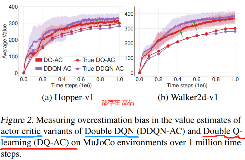
We measure the overestimation bias in Figure 2, which demonstrates that the actor-critic Double DQN suffers from a similar overestimation as DDPG (as shown in Figure 1).
我们在图 2 中测量了高估偏差，这证明 actor-critic Double DQN 遭受了与 DDPG 类似的高估 (如图 1 所示)。
While Double Q-learning is more effective, it does not entirely eliminate the overestimation.
虽然 Double Q-learning 更有效，但它并不能完全消除高估。
We further show this reduction is not sufficient experimentally in Section 6.1.
在第 6.1 节中，我们进一步在实验上证明这种减小是不够的

As ${\pi }_{{\varphi }_1}$ optimizes with respect to $Q_{{\theta }_1}$, using an independent estimate in the target update of $Q_{{\theta }_1}$ would avoid the bias introduced by the policy update.
由于 ${\pi }_{{\varphi }_1}$ 相对于 $Q_{{\theta }_1}$ 进行了优化，因此在 $Q_{{\theta }_1}$ 的目标更新中使用独立估计将避免策略更新引入的偏差。
However the critics are not entirely independent, due to the use of the opposite critic in the learning targets, as well as the same replay buffer.
然而，由于在学习目标中使用相反的 critic，以及相同的回放缓冲replay buffer ，critic 并非完全独立。
As a result, for some states $s$ we will have $Q_{{\theta }_2}(s,{\pi }_{{\varphi }_1}(s))>Q_{{\theta }_1}(s,{\pi }_{{\varphi }_1}(s))$.
因此，对于一些状态 $s$，我们将有 $Q_{{\theta }_2}(s,{\pi }_{{\varphi }_1}(s))>Q_{{\theta }_1}(s,{\pi }_{{\varphi }_1}(s))$。
This is problematic because $Q_{{\theta }_1}(s,{\pi }_{{\varphi }_1}(s))$ will generally overestimate the true value, and in certain areas of the state space the overestimation will be further exaggerated.
这是有问题的，因为 $Q_{{\theta }_1}(s,{\pi }_{{\varphi }_1}(s))$ 通常会高估真实价值，并且在状态空间的某些区域，高估会进一步被夸大。
To address this problem, we propose to simply upper-bound the less biased value estimate $Q_{{\theta }_2}$ by the biased estimate $Q_{{\theta }_1}$.
为了解决这个问题，我们提出通过有偏估计 $Q_{{\theta }_1}$ 简单地作为 偏差较小的价值估计 $Q_{{\theta }_2}$ 的上界。
This results in taking the minimum between the two estimates, to give the target update of our Clipped Double Q-learning algorithm:
由此取两个估计之间的最小值，从而给出我们的 Clipped Double Q-learning 算法的目标更新:
  ~  
$y_1=r+\gamma \underset{i=1,2}{\min }{Q}_{{\theta }_i^{\prime }}(s^{\prime },{\pi }_{{\varphi }_1}(s^{\prime }))(10)$
  ~  
With Clipped Double Q-learning, the value target cannot introduce any additional overestimation over using the standard Q-learning target.
使用 Clipped Double Q-learning，与使用标准 Q-learning 目标相比，价值目标不会引入任何额外的高估。
While this update rule may induce an underestimation bias, this is far preferable to overestimation bias, as unlike overestimated actions, the value of underestimated actions will not be explicitly propagated through the policy update.
虽然此更新规则可能导致低估偏差，但这比高估偏差要好得多，因为与高估的动作不同，低估的动作的价值不会通过策略更新显式传播。

In implementation, computational costs can be reduced by using a single actor optimized with respect to $Q_{{\theta }_1}$.
在实现中，可以通过使用相对于 $Q_{{\theta }_1}$ 优化的单个 actor 来减少计算成本。
We then use the same target $y_2=y_1$ for $Q_{{\theta }_2}$.
然后，我们对 $Q_{{\theta }_2}$ 使用相同的目标 $y_2=y_1$。
If $Q_{{\theta }_2}>Q_{{\theta }_1}$ then the update is identical to the standard update and induces no additional bias.
如果 $Q_{{\theta }_2}>Q_{{\theta }_1}$，则更新与标准更新相同，并且不会产生额外的偏差。
If $Q_{{\theta }_2}<Q_{{\theta }_1}$ , this suggests overestimation has occurred and the value is reduced similar to Double Q-learning.
如果 $Q_{{\theta }_2}<Q_{{\theta }_1}$，这表明发生了高估，并且价值减小了，类似于 Double Q-learning。
A proof of convergence in the finite MDP setting follows from this intuition.
在有限 MDP 设置下收敛性的证明是由这个直觉得出的。
We provide formal details and justification in the supplementary material.
我们在补充材料中提供了正式的细节和合理解释。

A secondary benefit is that by treating the function approximation error as a random variable we can see that the minimum operator should provide higher value to states with lower variance estimation error, as the expected minimum of a set of random variables decreases as the variance of the random variables increases.
第二个好处是，通过将函数近似误差视为随机变量，我们可以看到最小运算符应该为具有较低方差估计误差的状态提供更高的值，因为一组随机变量的最小值的期望 随着 随机变量方差的增加而 减小。
This effect means that the minimization in Equation (10) will lead to a preference for states with low-variance value estimates, leading to safer policy updates with stable learning targets.
这一效应意味着等式 (10) 中的最小化将导致对具有低方差价值估计的状态的偏好，从而导致具有稳定学习目标的更安全的策略更新。

5. 处理方差

While Section 4 deals with the contribution of variance to overestimation bias, we also argue that variance itself should be directly addressed.
虽然第 4 节处理方差对高估偏差的贡献，但我们也认为方差本身应该直接处理。
Besides the impact on overestimation bias, high variance estimates provide a noisy gradient for the policy update.
除了对高估偏差的影响外，高方差估计还为策略更新提供了噪声梯度。
This is known to reduce learning speed (Sutton & Barto, 1998) as well as hurt performance in practice.
众所周知，这会降低学习速度（Sutton & Barto, 1998），也会损害实践中的表现。
In this section we emphasize the importance of minimizing error at each update, build the connection between target networks and estimation error and propose modifications to the learning procedure of actor-critic for variance reduction.
在本节中，我们强调在每次更新时最小化误差的重要性，建立目标网络与估计误差之间的联系，并提出对 actor-critic 学习过程的修改以减小方差。

5.1. 累积误差

Due to the temporal difference update, where an estimate of the value function is built from an estimate of a subsequent state, there is a build up of error.
由于时序差分更新，其中对价值函数的估计是根据对后续状态的估计构建的，因此存在误差的累积。
While it is reasonable to expect small error for an individual update, these estimation errors can accumulate, resulting in the potential for large overestimation bias and suboptimal policy updates.
虽然预期单个更新的小误差是合理的，但这些估计误差会累积，导致潜在的严重高估偏差和次优策略更新。
This is exacerbated in a function approximation setting where the Bellman equation is never exactly satisfied, and each update leaves some amount of residual TD-error $\delta (s,a)$:
这在函数近似设置中会加剧，其中 Bellman 公式永远不会完全满足，并且每次更新都会留下一定量的残余 TD-error $\delta (s,a)$:
  ~  
$Q_{\theta }(s,a)=r+\gamma \mathbb{E}[Q_{\theta }(s^{\prime },a^{\prime })]-\delta (s,a)(11)$
  ~  
It can then be shown that rather than learning an estimate of the expected return, the value estimate approximates the expected return minus the expected discounted sum of future TD-errors:
然后可以证明，价值估计不是学习回报的期望的估计值，而是近似 $($回报的期望 $)$ 减去 $($ 未来 TD -误差的折扣和 的期望$)$:
  ~  
$\begin{array}{rl}{Q}_{\theta }(s_t,a_t)& =r_t+\gamma \mathbb{E}[Q_{\theta }(s_{t+1},a_{t+1})]-{\delta }_t\\ & =r_t+\gamma \mathbb{E}[r_{t+1}+\gamma \mathbb{E}[Q_{\theta }(s_{t+2},a_{t+2})]-{\delta }_{t+1}]-{\delta }_t\\ & ={\mathbb{E}}_{s_i\sim p_{\pi },a_i\sim \pi }[\sum _{i=t}^T{\gamma }^{i-t}(r_i-{\delta }_i)](12)\end{array}$
  ~  
If the value estimate is a function of future reward and estimation error, it follows that the variance of the estimate will be proportional to the variance of future reward and estimation error.
如果价值估计是未来奖励和估计误差的函数，则估计的方差将与未来奖励和估计误差的方差成正比。
Given a large discount factor $\gamma$, the variance can grow rapidly with each update if the error from each update is not tamed.
给定较大的折扣因子 $\gamma$，如果每次更新的误差不被控制，则方差可能随着每次更新而迅速增长。
Furthermore each gradient update only reduces error with respect to a small mini-batch which gives no guarantees about the size of errors in value estimates outside the mini-batch.
此外，每次梯度更新只能减小相对于小的 mini-batch 的误差，这不能保证减小在 mini-batch 之外的价值估计中误差的大小。

5.2. 目标网络 和 延迟策略更新

In this section we examine the relationship between target networks and function approximation error, and show the use of a stable target reduces the growth of error.
在本节中，我们研究目标网络和函数近似误差之间的关系，并证明使用稳定的目标可以降低误差的增长。
This insight allows us to consider the interplay between high variance estimates and policy performance, when designing reinforcement learning algorithms.
这种见解使我们能够在设计强化学习算法时考虑高方差估计和策略性能之间的相互作用。

Target networks are a well-known tool to achieve stability in deep reinforcement learning.
在深度强化学习中，目标网络是实现稳定性的一种众所周知的工具。
As deep function approximators require multiple gradient updates to converge, target networks provide a stable objective in the learning procedure, and allow a greater coverage of the training data.
由于深度函数近似器需要多个梯度更新才能收敛，目标网络在学习过程中提供了一个稳定的目标，允许更大范围的训练数据。
Without a fixed target, each update may leave residual error which will begin to accumulate.
没有固定的目标，每次更新可能会留下残余误差，这些误差将开始累积。
While the accumulation of error can be detrimental in itself, when paired with a policy maximizing over the value estimate, it can result in wildly divergent values.
误差的累积本身可能是有害的，当与最大化价值估计获得的策略相结合时，它会导致价值的巨大差异。

To provide some intuition, we examine the learning behavior with and without target networks on both the critic and actor in Figure 3, where we graph the value, in a similar manner to Figure 1, in the Hopper-v1 environment.
为了提供一些直觉，我们在图 3 中检查了 critic 和 actor 在有和没有目标网络的情况下的学习行为，我们在 Hopper-v1 环境中以类似于图 1 的方式绘制了价值。
In (a) we compare the behavior with a fixed policy and in (b) we examine the value estimates with a policy that continues to learn, trained with the current value estimate.
在 (a) 中，我们将行为与固定策略进行比较，在 (b) 中，我们检查 使用持续学习的，使用当前价值估计进行训练的策略估计的价值。
The target networks use a slow-moving update rate, parametrized by $\tau$.
目标网络使用缓慢移动的更新速率，通过 $\tau$ 参数化。

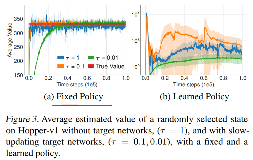
While updating the value estimate without target networks ($\tau =1$) increases the volatility, all update rates result in similar convergent behaviors when considering a fixed policy.
在没有目标网络 ($\tau =1$) 的情况下更新价值估计会增加波动性，但在考虑固定策略时，所有更新率都会导致类似的收敛行为。
However, when the policy is trained with the current value estimate, the use of fast-updating target networks results in highly divergent behavior.
然而，当使用当前价值估计来训练策略时，使用快速更新的目标网络会导致高度发散的行为。

When do actor-critic methods fail to learn?
什么时候 actor-critic 方法无法学习?
These results suggest that the divergence that occurs without target networks is the result of policy updates with a high variance value estimate.
这些结果表明，在没有目标网络的情况下发生的发散是具有高方差价值估计的策略更新的结果。
Figure 3, as well as Section 4, suggest failure can occur due to the interplay between the actor and critic updates.
图 3 和第 4 部分表明，由于 actor 和 critic 更新之间的相互作用，失败可能会发生。
Value estimates diverge through overestimation when the policy is poor, and the policy will become poor if the value estimate itself is inaccurate.
当策略差时，价值估计会因高估而发散，如果价值估计本身不准确，策略也会变得差。

If target networks can be used to reduce the error over multiple updates, and policy updates on high-error states cause divergent behavior, then the policy network should be updated at a lower frequency than the value network, to first minimize error before introducing a policy update.
如果目标网络可以用于减小多次更新的误差，并且高误差状态上的策略更新会导致不同的行为，那么 策略网络 应该以 比价值网络更低的频率更新，以便在引入策略更新之前首先最小化误差。
We propose delaying policy updates until the value error is as small as possible.
我们建议延迟策略更新，直到价值误差尽可能小。
The modification is to only update the policy and target networks after a fixed number of updates d to the critic.
改动在于 只在对 critic 进行固定次数的更新后 更新策略和目标网络。
To ensure the TD-error remains small, we update the target networks slowly ${\theta }^{\prime }\leftarrow \tau \theta +(1-\tau ){\theta }^{\prime }$.
为了确保 TD 误差很小，我们缓慢地更新目标网络 ${\theta }^{\prime }\leftarrow \tau \theta +(1-\tau ){\theta }^{\prime }$。
By sufficiently delaying the policy updates we limit the likelihood of repeating updates with respect to an unchanged critic.
通过充分延迟策略更新，我们限制了 针对未更改的 critic 重复更新的可能性。
The less frequent policy updates that do occur will use a value estimate with lower variance, and in principle, should result in higher quality policy updates.
确实发生的不太频繁的策略更新 将使用具有较低方差的价值估计，并且原则上应该导致更高质量的策略更新。
This creates a two-timescale algorithm, as often required for convergence in the linear setting (Konda & Tsitsiklis, 2003).
这创建了一个双时间尺度算法，通常需要在线性设置中收敛(Konda & Tsitsiklis, 2003)。
The effectiveness of this strategy is captured by our empirical results presented in Section 6.1, which show an improvement in performance while using fewer policy updates.
我们在第 6.1 节中提供的经验结果显示了该策略的有效性，证实在使用更少的策略更新的情况下，性能有所提高。

5.3. 目标策略平滑正则化

A concern with deterministic policies is they can overfit to narrow peaks in the value estimate.
确定性策略的一个问题是，它们会过拟合以缩小价值估计中的峰值。
When updating the critic, a learning target using a deterministic policy is highly susceptible to inaccuracies induced by function approximation error, increasing the variance of the target.
当更新 critic 时，使用确定性策略的学习目标极易受到函数近似误差引起的不准确性的影响，从而增加了目标的方差。
This induced variance can be reduced through regularization.
这种诱导方差可以通过正则化来减小。
We introduce a regularization strategy for deep value learning, target policy smoothing, which mimics the learning update from SARSA (Sutton & Barto, 1998).
我们为深度价值学习引入了一种正则化策略，即目标策略平滑，它模仿了 SARSA 的学习更新 (Sutton & Barto, 1998)。
Our approach enforces the notion that similar actions should have similar value.
我们的方法强化了类似的动作应该具有相近的价值的概念
While the function approximation does this implicitly, the relationship between similar actions can be forced explicitly by modifying the training procedure.
虽然函数近似隐式地做到了这一点，但可以通过修改训练过程显式地强制相似动作之间的关系。
We propose that fitting the value of a small area around the target action
我们提议拟合目标动作周围的一个小区域的价值
  ~  
$y=r+{\mathbb{E}}_{ϵ}[Q_{{\theta }^{\prime }}(s^{\prime },{\pi }_{{\varphi }^{\prime }}(s^{\prime })+ϵ)](13)$
  ~  
would have the benefit of smoothing the value estimate by bootstrapping off of similar state-action value estimates.
通过自举类似的状态-动作价值估计，将有利于平滑价值估计。
In practice, we can approximate this expectation over actions by adding a small amount of random noise to the target policy and averaging over mini-batches.
在实践中，我们可以通过向目标策略中添加少量随机噪声并对小批量进行平均来近似这种期望。
This makes our modified target update:
获得我们修改后的目标更新:
  ~  
$y=r+\gamma Q_{{\theta }^{\prime }}(s^{\prime },{\pi }_{{\varphi }^{\prime }}(s^{\prime })+ϵ)ϵ\sim \text{clip}(\mathcal{N}(0,\sigma ),-c,c)(14)$
  ~  
where the added noise is clipped to keep the target close to the original action.
其中添加的噪声被裁剪，以保持目标接近原始动作。
The outcome is an algorithm reminiscent of Expected SARSA (Van Seijen et al., 2009), where the value estimate is instead learned off-policy and the noise added to the target policy is chosen independently of the exploration policy.
结果是一种让人想起 Expected SARSA (Van Seijen et al.， 2009) 的算法，其中价值估计是异策略学习的off-policy ，并且添加到目标策略的噪声是独立于探索策略选择的。
The value estimate learned is with respect to a noisy policy defined by the parameter $\sigma$.
习得的价值估计是 关于 由参数 $\sigma$ 定义的噪声策略 的。

Intuitively, it is known that policies derived from SARSA value estimates tend to be safer, as they provide higher value to actions resistant to perturbations.
直觉上，我们知道，从 SARSA 价值估计中得出的策略往往更安全，因为它们为抵抗扰动的动作提供了更高的价值。
Thus, this style of update can additionally lead to improvement in stochastic domains with failure cases.
因此，这种更新方式可以额外地改善带有失败案例的随机域。
A similar idea was introduced concurrently by Nachum et al. (2018), smoothing over $Q_{\theta }$, rather than $Q_{{\theta }^{\prime }}$
Nachum 等人(2018) 同时引入了类似的想法，平滑 $Q_{\theta }$，而不是 $Q_{{\theta }^{\prime }}$

6. 实验

We present the Twin Delayed Deep Deterministic policy gradient algorithm (TD3), which builds on the Deep Deterministic Policy Gradient algorithm (DDPG) (Lillicrap et al., 2015) by applying the modifications described in Sections 4.2, 5.2 and 5.3 to increase the stability and performance with consideration of function approximation error.
我们提出了双延迟深度确定性策略梯度算法 (TD3)，该算法基于深度确定性策略梯度算法 (DDPG) (Lillicrap 等人，2015) ，通过应用第 4.2、5.2 和 5.3 节中描述的修改来提高稳定性和性能，同时考虑到函数近似误差。
TD3 maintains a pair of critics along with a single actor.
TD3 保留了两个 评论员critics 和一个 行为者actor。
For each time step, we update the pair of critics towards the minimum target value of actions selected by the target policy:
对于每个时间步，我们向目标策略选择的动作的最小目标价值 更新 评论员critics 对:
  ~  
$y=r+\gamma \underset{i=1,2}{\min }{Q}_{{\theta }_i^{\prime }}(s^{\prime },{\pi }_{{\varphi }^{\prime }}(s^{\prime })+ϵ)ϵ\sim \text{clip}(\mathcal{N}(0,\sigma ),-c,c)(15)$
  ~  
Every $d$ iterations, the policy is updated with respect to $Q_{{\theta }_1}$ following the deterministic policy gradient algorithm (Silver et al., 2014).
每 $d$ 次迭代，策略根据确定性策略梯度算法 (Silver et al.， 2014) 相对于 $Q_{{\theta }_1}$ 进行更新。
TD3 is summarized in Algorithm 1.
算法 1 总结了 TD3。

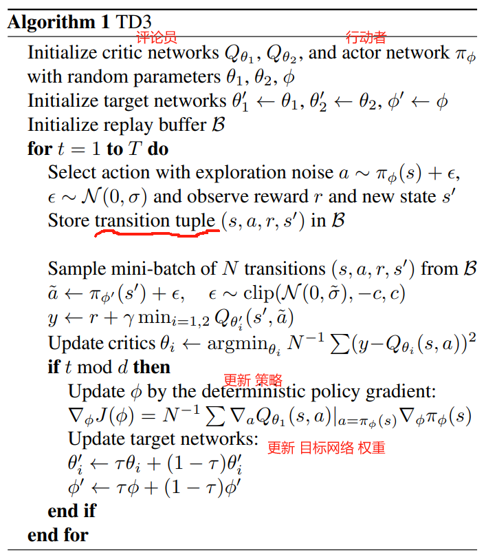
算法 1： TD3
用随机参数 ${\theta }_1,{\theta }_2,\varphi$ 初始化 critic 网络 $Q_{{\theta }_1},Q_{{\theta }_2}$ 和 actor 网络 ${\pi }_{\varphi }$
初始化目标网络 ${\theta }_1^{\prime }\leftarrow {\theta }_1$， ${\theta }_2^{\prime }\leftarrow {\theta }_2$，${\varphi }^{\prime }\leftarrow \varphi$
初始化回放缓冲区replay buffer $\mathcal{B}$
$\mathbf{for}t=1\mathbf{to}T\mathbf{do}$ 〔 时间步 〕
        ~~~~~~~        选择带有探索噪声的动作 $a\sim {\pi }_{\varphi }(s)+ϵ,ϵ\sim \mathcal{N}(0,\sigma )$
        ~~~~~~~        观测奖励 $r_t$ 和 新状态 $s^{\prime }$
        ~~~~~~~        存储转换元组 $(s_t,a_t,r_t,s_{t+1})$ 到 $\mathcal{B}$ 中
        ~~~~~~~        从 $\mathcal{B}$ 中抽取大小为 $N$ 的小批转换 $(s,a,r,s^{\prime })$
$\tilde{a}\leftarrow {\pi }_{{\varphi }^{\prime }}(s^{\prime })+ϵ,ϵ\sim \text{clip}(\mathcal{N}(0,\tilde{\sigma }),-c,c)$
$y\leftarrow r+\gamma \underset{i=1,2}{\min }{Q}_{{\theta }_i^{\prime }}(s^{\prime },\tilde{a})$
        ~~~~~~~        更新 critics： ${\theta }_i\leftarrow \frac{1}{N}\arg \underset{{\theta }_i}{\min }\sum (y-Q_{{\theta }_i}(s,a){)}^2$
$\mathbf{if}t\%d\mathbf{do}$
               ~~~~~~~~~~~~~~                通过确定性策略梯度 更新 $\varphi$：
${\nabla }_{\varphi }J(\varphi )=\frac{1}{N}\sum {\nabla }_a{Q}_{{\theta }_1}(s,a){|}_{a={\pi }_{\varphi }(s)}{\nabla }_{\varphi }{\pi }_{\varphi }(s)$ 〔 这里指定根据 critic 1 网络 (${\theta }_1$) 更新策略，SAC 取最小值 !!!〕 哪个更好呢？ ——> 算法当前的选择就是最好的
               ~~~~~~~~~~~~~~                更新目标网络： 〔 $\tau \ll 1$ 〕
${\theta }_i^{\prime }\leftarrow \tau {\theta }_i+(1-\tau ){\theta }_i^{\prime }$
${\varphi }^{\prime }\leftarrow \tau \varphi +(1-\tau ){\varphi }^{\prime }$
$\mathbf{end}\mathbf{if}$
$\mathbf{end}\mathbf{for}$

6.1. 评估

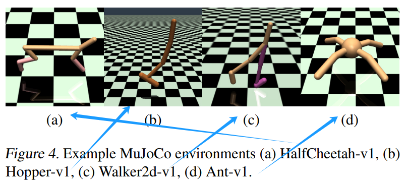
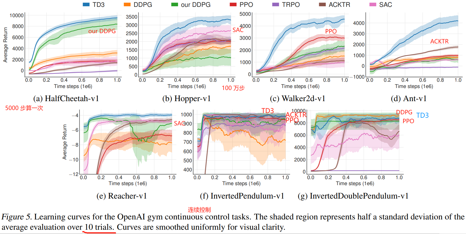
To evaluate our algorithm, we measure its performance on the suite of MuJoCo continuous control tasks (Todorov et al., 2012), interfaced through OpenAI Gym (Brockman et al., 2016) (Figure 4).
为了评估我们的算法，我们测量了它在通过 OpenAI Gym (Brockman et al.， 2016) 接口的 MuJoCo 连续控制任务套件上的性能 (Todorov等，2012)(图 4)。
To allow for reproducible comparison, we use the original set of tasks from Brockman et al. (2016) with no modifications to the environment or reward.
为了进行可重复的比较，我们使用了 Brockman 等人 (2016) 的原始任务集，没有对环境或奖励进行修改。

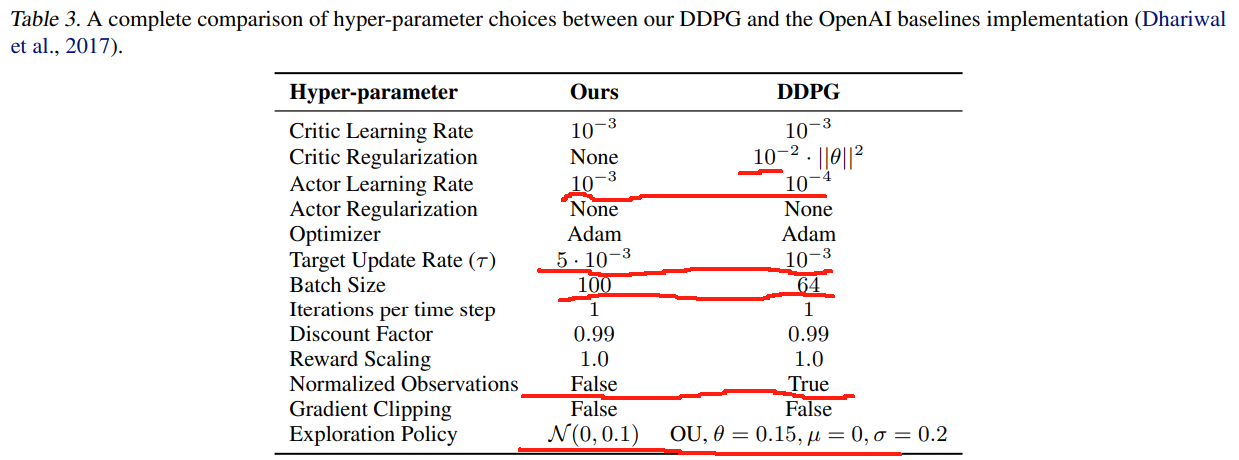
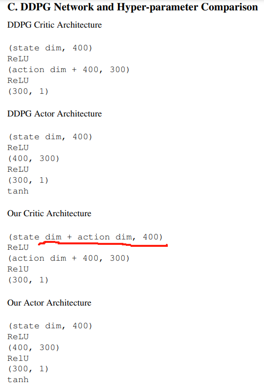
For our implementation of DDPG (Lillicrap et al., 2015), we use a two layer feedforward neural network of 400 and 300 hidden nodes respectively, with rectified linear units (ReLU) between each layer for both the actor and critic, and a final tanh unit following the output of the actor.
对于我们的 DDPG (Lillicrap等人，2015) 的实现，我们使用了一个两层前馈神经网络，分别包含 400 和 300 个隐藏节点，actor 和 critic 每层之间都有 修正线性单元 (ReLU)，以及 最终的 tanh 单元后是 actor 的输出。
Unlike the original DDPG, the critic receives both the state and action as input to the first layer.
与原始的 DDPG 不同的是，critic 同时接收状态和动作作为第一层的输入。
Both network parameters are updated using Adam (Kingma & Ba, 2014) with a learning rate of $10^{-3}$.
两个网络参数都使用 Adam (Kingma & Ba, 2014) 更新，学习率为 $10^{-3}$。
After each time step, the networks are trained with a mini-batch of a 100 transitions, sampled uniformly from a replay buffer containing the entire history of the agent.
在每个时间步之后，网络用 100 个转换transitions 的小批mini-batch 进行训练，这些转换从包含代理agent 整个历史的回放缓冲区replay buffer 中均匀采样。

The target policy smoothing is implemented by adding $ϵ\sim \mathcal{N}(0,0.2)$ to the actions chosen by the target actor network, clipped to $(-0.5,0.5)$, delayed policy updates consists of only updating the actor and target critic network every $d$ iterations, with $d=2$.
目标策略平滑 是通过将 $ϵ\sim \mathcal{N}(0,0.2)$ 添加到目标 actor 网络所选择的动作中来实现的，被裁剪为 $(-0.5,0.5)$，延迟策略更新包含 仅在每 $d$ 次迭代后更新 actor 和目标 critic 网络，使用 $d=2$。
While a larger $d$ would result in a larger benefit with respect to accumulating errors, for fair comparison, the critics are only trained once per time step, and training the actor for too few iterations would cripple learning.
虽然更大的 $d$ 会在累积误差方面带来更大的好处，但是为了公平的比较，每个时间步只训练一次 critics，并且训练 actor 的迭代次数太少会削弱学习。
Both target networks are updated with $\tau =0.005$.
两个目标网络都以 $\tau =0.005$ 更新。

To remove the dependency on the initial parameters of the policy we use a purely exploratory policy for the first 10000 time steps of stable length environments (HalfCheetah-v1 and Ant-v1) and the first 1000 time steps for the remaining environments.
为了消除对策略初始参数的依赖，我们对稳定长度环境 (HalfCheetah-v1 和 Ant-v1) 的前 10000 个时间步和其余环境的前 1000 个时间步使用纯探索性策略。
Afterwards, we use an off-policy exploration strategy, adding Gaussian noise $\mathcal{N}(0,0.1)$ to each action.
然后，我们使用一种异策略off-policy 探索策略，为每个动作添加高斯噪声 $\mathcal{N}(0,0.1)$。
Unlike the original implementation of DDPG, we used uncorrelated noise for exploration as we found noise drawn from the Ornstein-Uhlenbeck (Uhlenbeck & Ornstein, 1930) process offered no performance benefits.
与 DDPG 的原始实现不同，我们使用了非相关噪声进行探索，因为我们发现从 Ornstein-Uhlenbeck (Uhlenbeck & Ornstein, 1930) 过程中提取的噪声没有带来性能优势。

Each task is run for 1 million time steps with evaluations every 5000 time steps, where each evaluation reports the average reward over 10 episodes with no exploration noise.
每个任务运行 100 万个时间步，每 5000 个时间步评估一次，其中每个评估报告 没有探索噪声 的 10 个回合的平均奖励。
Our results are reported over 10 random seeds of the Gym simulator and the network initialization.
我们报告了 Gym 模拟器和网络初始化 的10 个随机种子 的结果。

We compare our algorithm against DDPG (Lillicrap et al., 2015) as well as the state of art policy gradient algorithms: PPO (Schulman et al., 2017), ACKTR (Wu et al., 2017) and TRPO (Schulman et al., 2015), as implemented by OpenAI’s baselines repository (Dhariwal et al., 2017), and SAC (Haarnoja et al., 2018), as implemented by the author’s GitHub1.
我们将我们的算法与 DDPG 以及最先进的策略梯度算法进行比较：PPO，ACKTR 和 TRPO (由 OpenAI 的基线数据库实现) 和 SAC，由作者的 GitHub 实现。

• 脚注 1 See the supplementary material for hyper-parameters and a discussion on the discrepancy in the reported results of SAC.
  参见关于超参数的补充材料和关于 SAC 报告结果差异的讨论。

Additionally, we compare our method with our re-tuned version of DDPG, which includes all architecture and hyper-parameter modifications to DDPG without any of our proposed adjustments.
此外，我们将我们的方法与重新调整的 DDPG 版本进行了比较，后者包括对 DDPG 的所有架构和超参数修改，而没有任何我们建议的调整。
A full comparison between our re-tuned version and the baselines DDPG is provided in the supplementary material.
我们重新调整的版本和基线 DDPG 之间的完整比较在补充材料中提供。

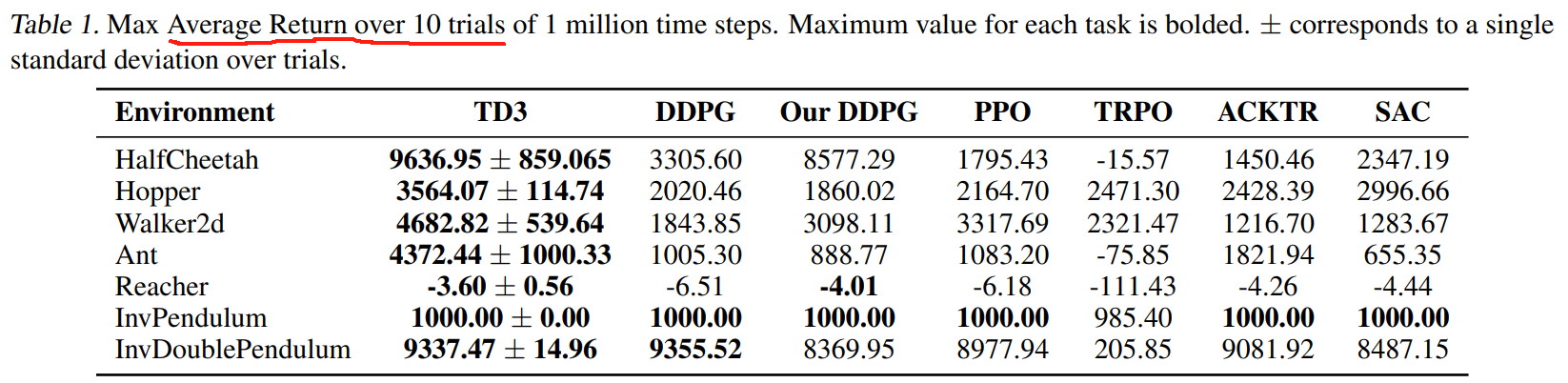
Our results are presented in Table 1 and learning curves in Figure 5.
我们的研究结果见表 1，学习曲线见图 5。
TD3 matches or outperforms all other algorithms in both final performance and learning speed across all tasks.
TD3 在所有任务的最终性能和学习速度上都与所有其他算法相匹配或优于其他算法。

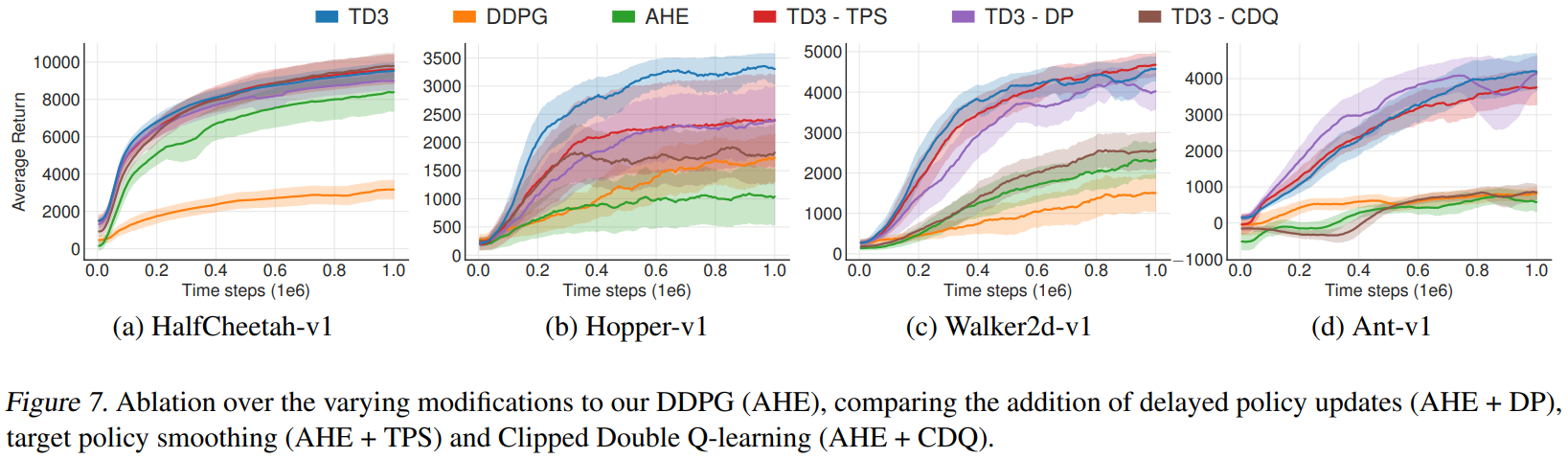
6.2. 消融研究

We perform ablation studies to understand the contribution of each individual component: Clipped Double Q-learning (Section 4.2), delayed policy updates (Section 5.2) and target policy smoothing (Section 5.3).
我们进行消融研究以了解每个单独组件的贡献：裁剪 Double Q-learning (第 4.2 节)，延迟策略更新 (第 5.2 节) 和目标策略平滑 (第 5.3 节)。
We present our results in Table 2 in which we compare the performance of removing each component from TD3 along with our modifications to the architecture and hyper-parameters.
我们在表 2 中展示了我们的结果，其中我们比较了从 TD3 中删除每个组件以及我们对架构和超参数的修改的性能。
Additional learning curves can be found in the supplementary material.
附加的学习曲线可以在补充材料中找到。

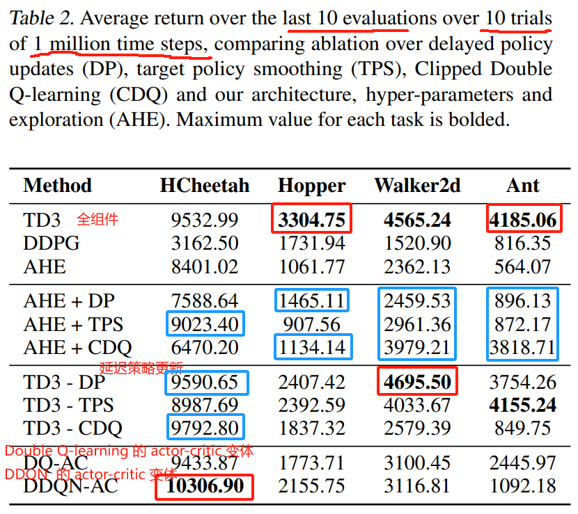
The significance of each component varies task to task.
每个组件的重要性因任务而异。
While the addition of only a single component causes insignificant improvement in most cases, the addition of combinations performs at a much higher level.
在大多数情况下，仅添加单个组件会带来微不足道的改进，但添加组合的效果要高得多。
The full algorithm outperforms every other combination in most tasks.
在大多数任务中，完整算法优于其他任何组合。
Although the actor is trained for only half the number of iterations, the inclusion of delayed policy update generally improves performance, while reducing training time.
尽管 actor 只训练了一半的迭代次数，但包含延迟策略更新通常会提高性能，同时减少训练时间。

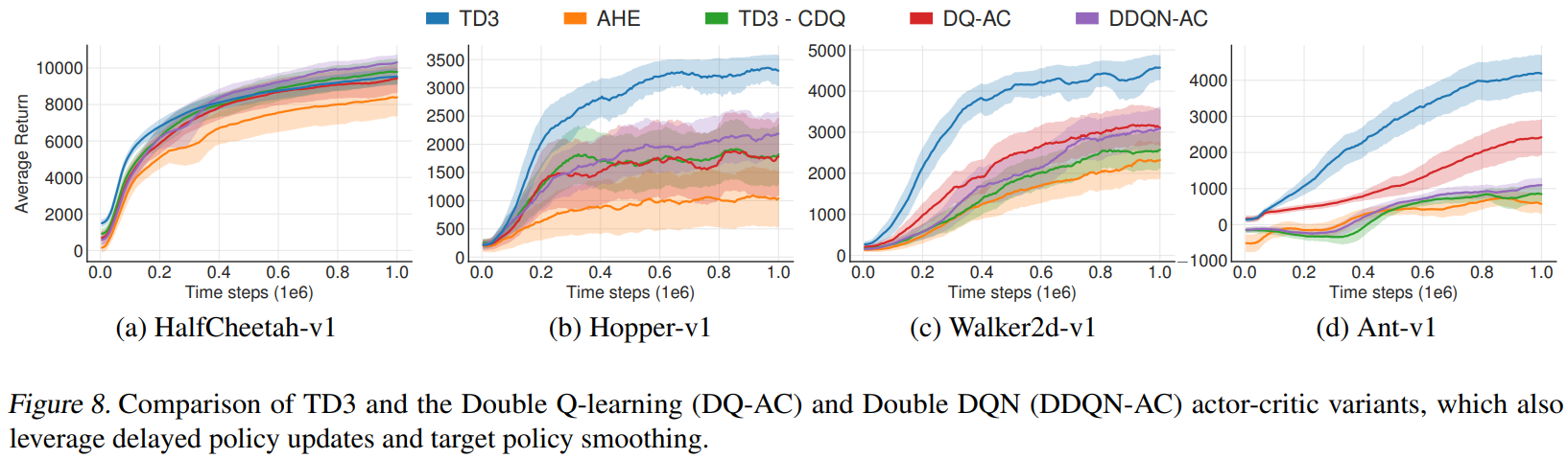
We additionally compare the effectiveness of the actor-critic variants of Double Q-learning (Van Hasselt, 2010) and Double DQN (Van Hasselt et al., 2016), denoted DQ-AC and DDQN-AC respectively, in Table 2.
我们还比较了 Double Q-learning (Van Hasselt, 2010) 和 Double DQN (Van Hasselt et al.， 2016) 的 actor-critic 变体的有效性，在表 2 中 分别记为 DQ-AC 和 DDQN-AC。
For fairness in comparison, these methods also benefited from delayed policy updates, target policy smoothing and use our architecture and hyper-parameters.
为了公平起见，这些方法还受益于延迟策略更新，目标策略平滑以及使用我们的架构和超参数。
Both methods were shown to reduce overestimation bias less than Clipped Double Q-learning in Section 4.
在第 4 节中，这两种方法都比 Clipped Double Q-learning 更能减少高估偏差。
This is reflected empirically, as both methods result in insignificant improvements over TD3 - CDQ, with an exception in the Ant-v1 environment, which appears to benefit greatly from any overestimation reduction.
这反映在经验上，因为这两种方法都比 TD3 - CDQ 产生了微不足道的改进，但在 Ant-v1 环境中例外，它似乎从任何高估的减少中受益匪浅。
As the inclusion of Clipped Double Q-learning into our full method outperforms both prior methods, this suggests that subduing the overestimations from the unbiased estimator is an effective measure to improve performance.
由于将 Clipped Double Q-learning 包含到我们的完整方法中，其性能优于之前的两种方法，这表明克服来自无偏估计量的高估是提高性能的有效措施。

7. 结论

Overestimation has been identified as a key problem in value-based methods.
In this paper, we establish overestimation bias is also problematic in actor-critic methods.
高估被认为是基于价值的方法中的一个关键问题。
在本文中，我们发现高估偏差在 actor-critic 方法中也是有问题的。
We find the common solutions for reducing overestimation bias in deep Q-learning with discrete actions are ineffective in an actor-critic setting, and develop a novel variant of Double Q-learning which limits possible overestimation.
我们发现用于离散动作的 deep Q-learning 中减少高估偏差的常见解决方案在 actor-critic 设置中是无效的，并开发了一种新的 Double Q-learning 变体，该变体限制了可能的高估。
Our results demonstrate that mitigating overestimation can greatly improve the performance of modern algorithms.
我们的结果表明，减轻高估可以大大提高新式算法的性能。

Due to the connection between noise and overestimation, we examine the accumulation of errors from temporal difference learning.
由于噪声和高估之间的联系，我们研究了时序差分学习的误差累积。
Our work investigates the importance of a standard technique in deep reinforcement learning, target networks, and examines their role in limiting errors from imprecise function approximation and stochastic optimization.
我们的工作研究了深度强化学习的一种标准技术 —— 目标网络的重要性，并研究了它们在限制来自不精确函数近似 和 随机优化的误差的作用。
Finally, we introduce a SARSA-style regularization technique which modifies the temporal difference target to bootstrap off similar state-action pairs.
最后，我们介绍了一种 SARSA 式的正则化技术，该技术修正了时序差分目标，以自举出相似的状态-动作对。

Taken together, these improvements define our proposed approach, the Twin Delayed Deep Deterministic policy gradient algorithm (TD3), which greatly improves both the learning speed and performance of DDPG in a number of challenging tasks in the continuous control setting.
总之，这些改进定义了我们提出的方法，双延迟深度确定性策略梯度算法 (TD3)，它大大提高了 DDPG 在连续控制设置中许多具有挑战性任务的学习速度和性能。
Our algorithm exceeds the performance of numerous state of the art algorithms.
我们的算法超越了许多最先进的算法的性能。
As our modifications are simple to implement, they can be easily added to any other actor-critic algorithm.
由于我们的修改很容易实现，因此可以很容易地将它们添加到任何其他 actor-critic 算法中。

参考文献

补充材料

• 下面的推导不是很清楚

A. 裁剪的 Double Q-Learning 收敛性证明

在有限 MDP 设置的 Clipped Double Q-learning 版本中，我们维护两个表格的价值估计 $Q^A$，$Q^B$。
在每个时间步，我们选择动作 $a^{\ast }=\arg {\max }_a{Q}^A(s,a)$，然后通过设置目标 $y$ 执行更新:
  ~  
$a^{\ast }=\arg \underset{a}{\max }{Q}^A(s^{\prime },a)$
  ~  
$y=r+\gamma \min (Q^A(s^{\prime },a^{\ast }),Q^B(s^{\prime },a^{\ast }))(16)$
  ~  
并更新关于目标和学习率 ${\alpha }_t(s,a)$ 的价值估计:
  ~  
$Q^A(s,a)=Q^A(s,a)+{\alpha }_t(s,a)(y-Q^A(s,a))$
  ~  
$Q^B(s,a)=Q^B(s,a)+{\alpha }_t(s,a)(y-Q^B(s,a))(17)$
  ~  
在有限 MDP 设置中，Double Q-learning 通常用于处理随机奖励或状态转换引起的噪声，因此 $Q^A$ 或 $Q^B$ 都是随机更新的。
然而，在函数近似设置中，兴趣可能更倾向于近似误差，因此我们可以在每次迭代中同时更新 $Q^A$ 和 $Q^B$。
这个证明自然延伸到随机更新。

该证明大量借鉴了 SARSA (Singh et al.， 2000) 以及 Double Q-learning (Van Hasselt, 2010) 的收敛性证明。
引理 1 的证明可以在 Singh 等人(2000) 中找到，他们建立在 Bertsekas(1995) 的一个命题之上。

引理 1： 考虑随机过程 $({\zeta }_t,{\Delta }_t,F_t),t\ge 0$， 其中 ${\zeta }_t,{\Delta }_t,F_t:X\to \mathbb{R}$ 满足等式：
  ~  
${\Delta }_{t+1}(x_t)=(1-{\zeta }_t(x_t)){\Delta }_t(x_t)+{\zeta }_t(x_t)F_t(x_t)(18)$
  ~  
其中 $x_t\in X$， 且 $t=0,1,2,...$
设 $P_t$ 为递增的 $\sigma$ 域序列，使得 ${\zeta }_0$ 和 ${∆}_0$ 是 $P_0$可测的， 且 ${\zeta }_t$，${∆}_t$ 和 $F_{t-1}$ 是 $P_t$ 可测的，$t=1,2,....$
假设下列情况成立:

1. 集合 $X$ 有限
2. ${\zeta }_t(x_t)\in [0,1]$，$\sum _t{\zeta }_t(x_t)=\infty$, $\sum _t({\zeta }_t(x_t){)}^2<\infty$， 以概率 1 且 $\forall x\ne x_t:\zeta (x)=0$
3. $\Vert \mathbb{E}[F_t|P_t]\Vert \le \kappa \Vert {\Delta }_t\Vert +c_t$， 其中 $\kappa \in [0,1)$， 且 $c_t$ 以概率 1 收敛到 0。
4. $\text{Var}[F_t(x_t)|P_t]\le K(1+\kappa \Vert {\Delta }_t\Vert {)}^2$， 其中 $K$ 为 某个常数。

• 其中 $\Vert \cdot \Vert$ 表示最大范数。
  然后 ${\Delta }_t$ 以 1 的概率收敛于 0。

定理 1： 给定以下条件：

1. 每个状态-动作对被采样无限次。
2. MDP 是有限的。
3. $\gamma \in [0,1)$
4. Q 值存储在一个查找表中
5. $Q^A$ 和 $Q^B$ 进行无限次更新。
6. 学习率 满足 ${\alpha }_t(s,a)\in [0,1]$， $\sum _t{\alpha }_t(s,a)=\infty$，$\sum _t({\alpha }_t(s,a){)}^2<\infty$， 以概率 1 且 ${\alpha }_t(s,a)=0,\forall (s,a)\ne (s_t,a_t)$
7. $\text{Var}[r(s,a)]<\infty ,\forall s,a$

那么 Clipped Double Q-learning 将以概率 1 收敛到 Bellman 最优公式定义的最优价值函数 $Q^{\ast }$。

定理 1 的证明：
将 引理 1 应用于 P t = { Q 0 A , Q 0 B , s 0 , a 0 , α 0 , r 1 , s 1 , ⋯   , s t , a t } P_t=\{Q_0^A,Q_0^B,s_0,a_0,\alpha_0,r_1,s_1,\cdots,s_t,a_t\} Pt​={Q0A​,Q0B​,s0​,a0​,α0​,r1​,s1​,⋯,st​,at​}，
$X=S\times A$，
${\Delta }_t=Q_t^A-Q^{\ast }$，
${\zeta }_t={\alpha }_t$
首先注意引理的条件 1 和条件 4 分别由定理的条件 2 和条件 7 成立。
引理条件 2 通过定理条件 6 和我们选择的 ${\zeta }_t={\alpha }_t$ 成立。
定义 $a^{\ast }=\arg {\max }_a{Q}^A(s_{t+1},a)$，有
  ~  
$\begin{array}{rl}{\Delta }_{t+1}(s_t,a_t)& =(1-{\alpha }_t(s_t,a_t))(Q_t^A(s_t,a_t)-Q^{\ast }(s_t,a_t))\\ & +{\alpha }_t(s_t,a_t)(r_t+\gamma \min (Q_t^A(s_{t+1},a^{\ast }),Q_t^B(s_{t+1},a^{\ast }))-Q^{\ast }(s_t,a_t))\\ & =(1-{\alpha }_t(s_t,a_t)){\Delta }_t(s_t,a_t)+{\alpha }_t(s_t,a_t)F_t(s_t,a_t)(19)\end{array}$
  ~  
其中 $F_t(s_t,a_t)$ 定义为：
  ~  
$\begin{array}{rl}{F}_t(s_t,a_t)& =r_t+\gamma \min (Q_t^A(s_{t+1},a^{\ast }),Q_t^B(s_{t+1},a^{\ast }))-Q^{\ast }(s_t,a_t)\\ & =r_t+\gamma \min (Q_t^A(s_{t+1},a^{\ast }),Q_t^B(s_{t+1},a^{\ast }))-Q^{\ast }(s_t,a_t)+\gamma Q_t^A(s_{t+1},a^{\ast })-\gamma Q_t^A(s_{t+1},a^{\ast })\\ & =F_t^Q(s_t,a_t)+c_t(20)\end{array}$
  ~  
其中 $F_t^Q(s_t,a_t)=r_t+\gamma Q_t^A(s_{t+1},a^{\ast })-Q^{\ast }(s_t,a_t)$， 表示 标准 Q-learning 中 $F_t$ 的价值
$c_t=\gamma \min (Q_t^A(s_{t+1},a^{\ast }),Q_t^B(s_{t+1},a^{\ast }))-\gamma Q_t^A(s_{t+1},a^{\ast })$
  ~  
由于 $\mathbb{E}[F_t^Q|P_t]\le \gamma \Vert {\Delta }_t\Vert$ 是已知的，如果 $c_t$ 以概率 1 收敛到 0， 则 引理 1 的条件 3 成立。
——————————————
假设 $y=r_t+\gamma \min (Q_t^A(s_{t+1},a^{\ast }),Q_t^B(s_{t+1},a^{\ast }))$， 且 ${\Delta }_t^{BA}(s_t,a_t)=Q_t^B(s_t,a_t)-Q_t^A(s_t,a_t)$，
如果 ${\Delta }^{BA}$ 收敛到 0， 则 $c_t$ 收敛到 0。
时间 $t$ 处的 ${\Delta }^{BA}$ 更新为 $Q^A$ 和 $Q^B$ 更新的和：
  ~  
$\begin{array}{rl}{\Delta }_{t+1}^{BA}(s_t,a_t)& ={\Delta }_t^{BA}(s_t,a_t)+{\alpha }_t(s_t,a_t)(y-Q_t^B(s_t,a_t)-(y-Q_t^A(s_t,a_t)))\\ & ={\Delta }_t^{BA}(s_t,a_t)+{\alpha }_t(s_t,a_t)(Q_t^A(s_t,a_t)-Q_t^B(s_t,a_t))\\ & =(1-{\alpha }_t(s_t,a_t)){\Delta }_t^{BA}(s_t,a_t)(21)\end{array}$
  ~  
显然，${\Delta }_t^{BA}$ 将收敛于 0，这表明我们已经满足引理 1 的条件 3，这意味着 $Q^A(s_t,a_t)$ 收敛于 $Q_t^{\ast }(s_t,a_t)$。
同样，我们通过选择 $Q_t^B-Q^{\ast }$ 并重复相同的参数，得到 $Q^B(s_t,a_t)$ 收敛于最优价值函数，从而证明定理 1。

B. 确定性策略梯度的高估偏差

If the gradients from the deterministic policy gradient update are unnormalized, this overestimation is still guaranteed to occur under a slightly stronger condition on the expectation of the value estimate.
如果来自确定性策略梯度更新的梯度是非标准化的，那么在对价值估计的期望稍强的条件下，仍然肯定会出现这种高估。
Assume the approximate value function is equal to the true value function, in expectation over the steady-state distribution, with respect to policy parameters between the original policy and in the direction of the true policy update:
假设近似价值函数等于真正的价值函数，在稳态分布的期望中，对于原策略和真策略更新方向之间的策略参数:
  ~  
${\mathbb{E}}_{s\sim \pi }\left[Q_{\theta }\right(s,{\pi }_{\text{new}}(s)\left)\right]={\mathbb{E}}_{s\sim \pi }\left[Q^{\pi }\right(s,{\pi }_{\text{new}}(s)\left)\right](22)$
  ~  
$\forall {\varphi }_{\text{new}}\in [\varphi ,\varphi +\beta ({\varphi }_{\text{true}}-\varphi )]$ 使得 $\beta >0$
  ~  
注意到 ${\varphi }_{\text{true}}$ 最大化真正价值的变化率 ${\Delta }_{\text{true}}^{\pi }=Q^{\pi }(s,{\pi }_{\text{true}}(s))-Q^{\pi }(s,{\pi }_{\varphi }(s))$， ${\Delta }_{\text{true}}^{\pi }\ge {\Delta }_{\text{аpprox}}^{\pi }$。
给定条件 22，近似价值的最大变化率必须至少一样大 ${\Delta }_{\text{approx}}^{\theta }\ge {\Delta }_{\text{true}}^{\pi }$。
给定 $Q_{\theta }(s,{\pi }_{\varphi })=Q^{\pi }(s,{\pi }_{\varphi })$，这意味着 $Q_{\theta }(s,{\pi }_{\text{approx}}(s))\ge Q^{\pi }(s,{\pi }_{\text{true}}(s))\ge Q^{\pi }(s,{\pi }_{\text{approx}}(s))$，显示了价值函数的高估。

C. DDPG 网络 和 超参数比较

D. 附加的实现细节

For clarity in presentation, certain implementation details were omitted, which we describe here.
为了表述清晰，省略了某些实现细节，我们在这里描述。
For the most complete possible description of the algorithm, code can be found on our GitHub (https://github.com/sfujim/TD3).
对于最完整的算法描述，可以在我们的 GitHub (https://github.com/sfujim/TD3) 上找到代码。

Our implementation of both DDPG and TD3 follows a standard practice in deep Q-learning, in which the update differs for terminal transitions.
我们对 DDPG 和 TD3 的实现遵循了 deep Q-learning 的标准实践，其中终止转换的更新是不同的。
For transitions where the episode terminates by reaching some failure state, and not due to the episode running until the max horizon, the value of $Q(s,\cdot )$ is set to 0 in the target $y$:
对于在到达某个失败状态而不是由于回合运行直到最大视界的回合终止的转换transitions ，$Q(s，\cdot )$ 的值在目标 $y$ 中被设置为0:
  ~  
$f=\{\begin{array}{rl}& r\text{if terminal }{s}^{\prime }\text{and }t<\max \text{horizon}\\ & r+\gamma Q_{{\theta }^{\prime }}(s^{\prime },{\pi }_{{\varphi }^{\prime }}(s^{\prime })\text{else}\end{array}$
  ~  
For target policy smoothing (Section 5.3), the added noise is clipped to the range of possible actions, to avoid error introduced by using values of impossible actions:
对于目标策略平滑(第 5.3 节)，添加的噪声被裁剪到可能动作的范围内，以避免使用不可能动作的值带来的误差:
  ~  
$y=r+\gamma Q_{{\theta }^{\prime }}(s^{\prime },\text{clip}({\pi }_{{\varphi }^{\prime }}(s^{\prime }),\text{min action},\text{max action}\left)\right)$
  ~  
$ϵ\sim \text{clip}(\mathcal{N}(0,\sigma ),-c,c)$

E. Soft Actor-Critic 实现细节

For our implementation of Soft Actor-Critic (Haarnoja et al., 2018) we use the code provided by the author (https: //github.com/haarnoja/sac), using the hyper-parameters described by the paper.
对于我们的 Soft Actor-Critic (Haarnoja 等人，2018) 的实现，我们使用作者提供的代码 (https: //github.com/haarnoja/sac)，使用论文描述的超参数。
We use a Gaussian mixture policy with 4 Gaussian distributions, except for the Reacher-v1 task, where we use a single Gaussian distribution due to numerical instability issues in the provided implementation.
我们使用具有 4 个高斯分布的高斯混合策略，除了 Reacher-v1 任务，由于提供的实现中的数值不稳定性问题，我们使用单个高斯分布。
We use the environment-dependent reward scaling as described by the authors, multiplying the rewards by 3 for Walker2d-v1 and Ant-v1, and 1 for all remaining environments.
我们使用作者所描述的环境相关奖励缩放比例，将 Walker2d-v1 和 Ant-v1 的奖励乘以 3，将所有剩余环境的奖励乘以 1。

For fair comparison with our method, we train for only 1 iteration per time step, rather than the 4 iterations used by the results reported by the authors.
为了与我们的方法进行公平的比较，我们每个时间步只训练 1 次迭代，而不是作者报告的结果所使用的 4 次迭代。
This along with fewer total time steps should explain for the discrepancy in results on some of the environments.
加上更少的总时间步，这应该可以解释在某些环境中结果的差异
Additionally, we note this comparison is against a prior version of Soft Actor-Critic, while the most recent variant includes our Clipped Double Q-learning in the value update and produces competitive results to TD3 on most tasks.
此外，我们注意到这种比较是针对先前版本的 Soft Actor-Critic，而最新的版本包括我们在价值更新中的 Clipped Double Q-learning，并在大多数任务上产生与 TD3 有竞争力的结果。

F. 附加的 学习曲线