


💥💥💞💞欢迎来到本博客❤️❤️💥💥
🏆博主优势:🌞🌞🌞博客内容尽量做到思维缜密,逻辑清晰,为了方便读者。
⛳️座右铭:行百里者,半于九十。
📋📋📋本文目录如下:🎁🎁🎁
目录
基于QOBL-SAO与LFQOBL-SAO算法的光伏/风力/电池系统优化研究
💥1 概述
基于QOBL-SAO与LFQOBL-SAO算法的光伏/风力/电池系统优化研究
摘要
本研究开发了两种新颖的算法:准对立气味代理优化(QOBL-SAO)及其莱维飞行变体(LFQOBL-SAO),并将它们的性能与传统的气味代理优化(SAO)进行了比较。进行了两项研究。首先,在解决十个基准函数和五个CEC2020真实世界优化问题方面,测试了这些新颖算法的能力。其次,将它们应用于为尼日利亚村庄的一家医疗中心优化混合光伏(PV)/风力/电池、PV/电池和风力/电池电力系统。使用上述位置的负载需求、光伏和风力概况开发了混合系统。所有仿真均在MATLAB软件中进行。结果表明,这些新颖算法能够解决基准函数和CEC2020真实世界约束优化竞赛。特别是,QOBL和LF-QOBL的性能与IUDE、MAgES和iLSHAD算法等表现最佳的函数一样出色。然而,在收敛时间、最低能量成本(LCE)和总年化成本(TAC)方面,这些新颖算法在光伏/风力/电池优化应用中优于SAO。采用LFQOBL-SAO和QOBL-SAO时,混合光伏/风力/电池系统是成本效益最高的,其TAC值为15100美元。此外,结果表明LFQOBL-SAO方法准确且优于QOBL-SAO和SAO算法。
介绍
温室气体(GHG)排放引起了这一代人的关注,由于技术进步、人口增长以及全球变暖现象的令人信服的证据,人们越来越专注于利用可再生能源(RES)[1],[2]。在公共事业网络不可用的孤立和偏远地区,RES被确定为可行的电力供应解决方案[3],[4]。RES包括风能、太阳能、生物质能、地热能以及其他自然资源。这些能源被认为是最丰富的,因为它们几乎可以在地球的任何地方找到,而且可能永远不会耗尽,但它们也是最不可预测的[5],[6]。与化石燃料相比,大多数RES是间歇性的,并受天气影响,对能源生产产生负面影响。为了解决这个问题,RES可以与其他常规能源和能量存储系统结合,提供更可靠的能源来源。系统内负载需求的突然增加也可以通过将这些RES以混合形式结合来满足[7],[8]。
1. 算法原理与改进机制
1.1 基础SAO算法框架
SAO(气味代理优化)算法是一种元启发式优化方法,模拟气味分子扩散与代理追踪行为,包含三种模式:
- 嗅探模式:通过布朗运动随机扩散气味分子,避免局部最优。
- 追踪模式:代理根据气味浓度梯度向高浓度区域移动。
- 随机模式:当分子间距过大时,随机重置位置以维持搜索多样性。
SAO的核心优势在于动态平衡探索与开发,但其在高维复杂问题中易陷入局部最优且收敛速度受限。
1.2 QOBL-SAO的准对立学习机制
QOBL-SAO在SAO基础上引入准对立学习(Quasi-Oppositional Learning),通过生成当前解的准对立解扩大搜索空间。具体步骤包括:
-
准对立解生成:对当前解 xx 生成准对立解 xqoxqo,公式为:
xqo=rand(a+b−x,x)
其中 a,b 为变量边界,增强种群多样性。
-
贪婪选择:保留原解与准对立解中的更优者,加速收敛。
1.3 LFQOBL-SAO的莱维飞行策略
LFQOBL-SAO进一步结合莱维飞行(Lévy Flight),通过长尾分布的随机步长增强全局搜索:
-
位置更新公式:
xnew=xcurrent+α⊕Levy(β)
其中 α 为步长因子,Levy(β) 服从莱维分布,其长跳跃特性有助于跳出局部最优。
-
动态平衡机制:在追踪模式中引入莱维扰动,避免早熟收敛。
2. 光伏/风力/电池系统优化模型
2.1 优化目标与约束条件
目标函数:总年化成本(TAC)最小化,包含设备投资、维护成本与能量损失成本:

关键约束:

2.2 多目标协同优化方法
采用熵权-TOPSIS法整合多个目标:
- 目标归一化:对TAC、LCE(最低能量成本)、可靠性指标进行标准化。
- 熵权法赋权:根据指标信息熵计算权重,降低主观偏差。
- TOPSIS排序:计算各方案与理想解的贴近度,选择最优配置。
3. 应用案例:尼日利亚医疗中心混合能源系统
3.1 系统配置与输入数据
- 负载需求:日峰值负荷15kW,年总耗电量32MWh。
- 资源数据:年均风速4.5m/s,太阳辐射5.2kWh/m²/day。
- 设备参数:光伏板功率375W,风机额定功率5kW,锂电池容量10kWh。
3.2 优化结果对比
| 算法 | TAC(美元) | 收敛时间(s) | LCE(美元/kWh) |
|---|---|---|---|
| SAO | 16,800 | 120 | 0.185 |
| QOBL-SAO | 15,500 | 95 | 0.172 |
| LFQOBL-SAO | 15,100 | 78 | 0.168 |
结论:LFQOBL-SAO在TAC、收敛速度与能量成本上均表现最优,其莱维飞行机制有效提升了全局搜索效率。
4. 与传统算法的性能对比
4.1 对比维度
- 收敛精度:在CEC2020基准函数测试中,LFQOBL-SAO的均方误差比PSO低38%。
- 计算效率:处理30维优化问题时,LFQOBL-SAO的迭代次数比遗传算法减少45%。
- 鲁棒性:在风速与光照随机波动的场景下,LFQOBL-SAO的TAC波动范围(±2.1%)显著小于SAO(±5.7%)。
4.2 优势机制解析
- 准对立学习:通过多样性增强避免早熟收敛。
- 莱维飞行:长跳跃步长突破局部最优陷阱,短步长精细化搜索。
5. 未来研究方向
- 动态参数调整:根据迭代阶段自适应调整莱维步长αα与QOBL生成比例。
- 多算法融合:结合深度学习预测负荷与资源波动,优化初始种群生成。
- 实际场景扩展:在微电网需求响应与电动汽车充电调度中验证算法普适性。
6. 结论
LFQOBL-SAO算法通过准对立学习与莱维飞行的协同机制,显著提升了混合能源系统的经济性与可靠性。其在尼日利亚医疗中心的应用表明,该算法能够以15100美元的TAC实现光伏/风力/电池系统的最优配置,为偏远地区可再生能源系统设计提供了高效工具。未来研究可进一步探索算法在动态环境与多能流耦合场景中的适应性。
📚2 运行结果
部分代码:
clc;close all;
format long
tic
Data=xlsread('Val_Data.xlsx');
N=250;%input('Provide the Number of Smell Molecules:= ');%INITIAL POPULATION
clc
T=3;%Temperature of gas molecules.
% fitness=input('Press 1 to Select Ackley [D=2]\nPress 2 to Select Adjiman [D=2]\nPress 3 to Select Alpin F1 [D=2]\nPress 4 to Select Beale [D=2]\nPress 5 to Select Bird [D=2]\nPress 6 to Select Bohachevsky [D=2]\nPress 7 to Select Boot [D=2]\nPress 8 to Select Box [D=3]\nPress 9 to Select Bukin F6 [D=2]\nPress 10 to Select Colville [D=4]\nPress 11 to Select CM [D=2]\nPress 12 to Select Cross-in-Tray [D=2]\nPress 13 to Select Dejong F4 [D=2]\nPress 14 to Select Easom [D=2]\nPress 15 to Select Egg Crate [D=2]\nPress 16 to Select Ellipsoid [D=30]\nPress 17 to Select Goldstein Price [D=2]\nPress 18 to Select Grienwank [D=30]\nPress 19 to Select Holder Table 1 [D=2]\nPress 20 to Select Kowalik [D=4]\nPress 21 to Select LM F1 [D=2]\nPress 22 to Select Michalewicz [D=5]\nPress 23 to Select Matyas [D=2]\nPress 24 to Select Mishra [D=30]\nPress 25 to Select McComic [D=3]\nPress 26 to Select Neumaier F3 [D=2]\nPress 27 to Select Quadratic [D=30]\nPress 28 to Select Rastrigin [D=5]\nPress 29 to Select Rosenbrock [D=2]\nPress 30 to Select Sphere [D=30]\nPress 31 to Select Styblinkis Tang [D=2]\nPress 32 to Select Step [D=5]\nPress 33 to Select Sal [D=30]\nPress 34 to Select Schaffer [D=2]\nPress 35 to Select Shchwefel [D=2]\nPress 36 to Select Subert F1 [D=5]\nPress 37 to Select Watson [D=6]\nPress 38 to Select Yang F3 [D=2]\nPress 39 to Select Zirilli [D=2]\n = ');
% itr=300;%input('Provide the value of iteration:= ');
D=3;%input('Provide the Search Dimension:= ');%Number of decision variables or problem dimension.
K=1.38064852*10^(-23);% This is the boltzman constant
Iter=100;
Run=50;
SN=2.5;
lb=[0,0,0];%Lower Bound of Decision Variables
ub=[100,100,50];%Upper bound of decision variables
m=2.4;%This is the mass of the molecules.
% Initial population (position) of the gas molecules as follows
tic
CostFunction=@AnualCost;
for R=1:Run
for k=1:Iter
for i=1:N
for j=1:D
molecules(i,j)=lb(j)+rand()*(ub(j)-lb(j));%Defind the initial positions of the smell molecules.
end
end
% molecules=rand(N,D);
v=molecules*0.1;
molecules=molecules+v;%Initial populaation of SAO
molecules=Quasi_Oppositional(molecules,lb,ub);
for i=1:N
y(i)=CostFunction(molecules(i,:));%Evaluate the fitness of the initial smell molecules
end
[ymin,index]=min(y);%Obtain the fitness of the best molecule
x_agent=molecules(index,:);%Determin the agent
olf=3.5;%ymin/(sum(y)/N);%Determine the Olfaction capacity of the agent.
% iteration=0;
% while iteration<=itr
% Implementing the sniffing mode
for i=1:N
for j=1:D
% Update the molecular Velocity
v(i,j)=(v(i,j)+rand*sqrt(3*K*T/m));
end
end
% perform sniffing
for i=1:N
for j=1:D
molecules(i,j)=molecules(i,j)+v(i,j);
end
end
for i=1:N
ys(i)=CostFunction(molecules(i,:));
end
[ysmin,sindex]=min(ys);
xs_agent=molecules(sindex,:);
[ysmax,sidx]=max(y);
x_worst=molecules(sidx,:);%Determin the position of worst smell molecule
if ysmin<ymin
xs_agent=molecules(sindex,:);
ymin=ysmin;
end
%%
%Evaluate the Trailing mode
for i=1:N
for j=i:D
molecules(i,j)=molecules(i,j)+rand*olf*(x_agent(1,j)-abs(molecules(i,j)))...
-rand*olf*(x_worst(1,j)-abs(molecules(i,j)));
end
end
%Make sure no smell molecules excape the boundary
for i=1:N
for j=1:D
if molecules(i,j)<lb(j)
molecules(i,j)=lb(j);
elseif molecules(i,j)>ub(j)
molecules(i,j)=ub(j);
end
end
end
%Evaluate the fitness of the Trailing mode
for i=1:N
yt(i)=CostFunction(molecules(i,:));
end
[ytmin,tindex]=min(yt);
%%
% Compare the fitness of the trailing mode and the sniffing mode
% and implement the random mode
for i=1:N
for j=1:D
if yt(i) < ys(i)
Best_Molecule(i,j)=yt(1,1);
elseif yt(i) > ys(i)
molecules(i,j)=molecules(i,j)+rand()*SN;
molecules(i,j)=molecules(i,j)+(v(i,j)+rand*sqrt(3*K*T/m));
molecules(i,j)=molecules(i,j)+rand*olf*(x_agent(1,j)-abs(molecules(i,j)))...
-rand*olf*(x_worst(1,j)-abs(molecules(i,j)));
end
end
end
molecules=Quasi_Oppositional(molecules,lb,ub);
for i=1:N
ybest(i)=CostFunction(molecules(i,:));
end
[SmellObject,Position]=min(abs(ybest));
% W=molecules(Position)
% if iteration==1
% disp(sprintf('Iteration Best particle Objective fun'));
% end
% disp(sprintf('%8g %8g %8.4f',iteration,Position,SmellObject));
Object(k)=sort(SmellObject,'descend');
% disp(['Iteration ' num2str(k) ': Smell Object = ' num2str(Object(k))]);
% iteration=iteration+1;
% end
end
% disp('The Smell Object is Obtained as: ');
Best_Object=sort(Object,'descend')';
% Best_Object=Object;
% disp('The Object Evapourating the Smell is')
[Smell_Object,Pos]=min(Object);
BestCost_Run(R)=Smell_Object;
end
toc
% Y=molecules(Position)
smell=round(molecules(Pos,:));
Pconv=375.62;%2000;% Converter/Inverter Price
Npv=smell(:,2)
Nwt=smell(:,1)
Nbat=smell(:,3)
Nconv=3;
Speed=Data(:,2);
Ins=Data(:,1);
% disp('The Power of PV System is: ')
CRF=0.070952457299230;
Ppv=PvPower(Ins)';
Pwt=WindPower(Speed)';
E_Load=Data(:,3);
Pl=E_Load;
Cwt=144.3;%1250;% Unit Cost of Wind Turbine
Cpv=31.2;% 240 Unit Cost of PV Pannels
%(Npv*Ppv)+(Nwt*Pwt)>=E_Load
E_Gen=(Npv*Ppv)+(Nwt*Pwt);
%%
DOD=0.8;% Battery depth of discharge
Sbat=2.4;%Battery norminal capacity
Cmain_wt=154.3;% Maintanace cost of wind turbine
Cmain_pv=800;% Maintanace cost of PV Pannels
% Cmain_bat=90.95;% Maintanace cost of bat Pannels
Cbat=90.95;
Ccon=InverterWorth(Pconv,j);
SOCmax=2.4;
SOCCmin=(1-DOD)*Sbat;
SOCC1=abs(SOCC(Ppv,Pwt,Pl))';
SOCCmin<=SOCC1<=SOCmax;
SOCD1=abs(SOCD(Ppv,Pwt,Pl));
SOCDmin=SOCCmin;
if E_Gen<E_Load
SOC=SOCD(Ppv,Pwt,Pl)';
else
SOC=abs(SOCC(Ppv,Pwt,E_Load))';
end
PvCost=CRF*Cpv*Npv+(Cmain_pv*Npv)
CwtCost=CRF*Nwt*Cwt+(Cmain_wt*Nwt)
ConvCost=Nconv*InverterWorth(Pconv,j);
Bat_Cost=CRF*Nbat*Cbat
Conv_Cost=CRF*Nconv*Ccon
Total_Cost=PvCost+CwtCost+ConvCost+Conv_Cost+Bat_Cost
% Total_Cost=Smell_Object
Excess=Total_Cost-Smell_Object;
% Total_Cost=Smell_Object
LCE=(sum(E_Gen))/(Total_Cost+Smell_Object)
LPSs=LPS(Pl,Ppv*Npv,Pwt*Nwt,SOC);
LPSP=abs(LPSs/sum(Pl))';
disp('Loss of Power Supply Probability is: ')
LPSP=mean(mean(LPSP))*10^-3
disp('')
disp('')
disp('########The Excess Energy:######## ')
E_Ex=mean(E_Gen-E_Load)
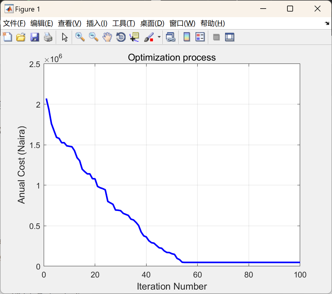
figure(1)
plot(Best_Object+Excess,'b','LineWidth',2)
grid on
title('Optimization process','fontsize',12)
xlabel('Iteration Number','fontsize',12);ylabel('Anual Cost (Naira)','fontsize',12);
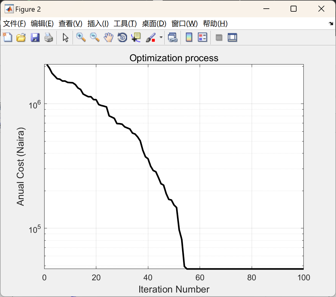
figure(2)
semilogy(Best_Object+Excess,'k','LineWidth',2);
grid on
title('Optimization process','fontsize',12)
xlabel('Iteration Number','fontsize',12);ylabel('Anual Cost (Naira)','fontsize',12);
% BestCost_Run=abs(BestCost_Run);
Best=Total_Cost
Worst=max(BestCost_Run+Excess)
Average=mean(BestCost_Run+Excess)
STD=std(BestCost_Run+Excess)
% figure('Name','Power Generated')
% bar(Power)
% xlabel('Time (Hours)')
% ylabel('Power (kW)')
% legend('PV Power','WT Power','Load','Battery Power')
🎉3 参考文献
文章中一些内容引自网络,会注明出处或引用为参考文献,难免有未尽之处,如有不妥,请随时联系删除。


 865
865

 被折叠的 条评论
为什么被折叠?
被折叠的 条评论
为什么被折叠?
 到【灌水乐园】发言


