基于MATLAB中雷达和视觉合成数据的目标级传感器融合（Matlab代码实现）-CSDN博客

本文链接：https://blog.csdn.net/weixin_46039719/article/details/147645572

👨‍🎓个人主页

💥💥💞💞欢迎来到本博客❤️❤️💥💥

🏆博主优势：🌞🌞🌞博客内容尽量做到思维缜密，逻辑清晰，为了方便读者。

⛳️座右铭：行百里者，半于九十。

📋📋📋本文目录如下：🎁🎁🎁

目录

💥1 概述

一、引言

二、研究背景与意义

三、融合方法与技术

四、研究内容与实现

五、仿真实验与结果分析

六、结论与展望

📚2 运行结果

🎉3 参考文献

🌈4 Matlab代码实现

💥1 概述

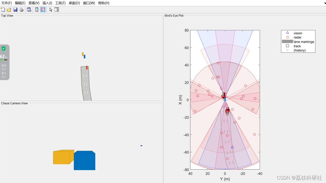
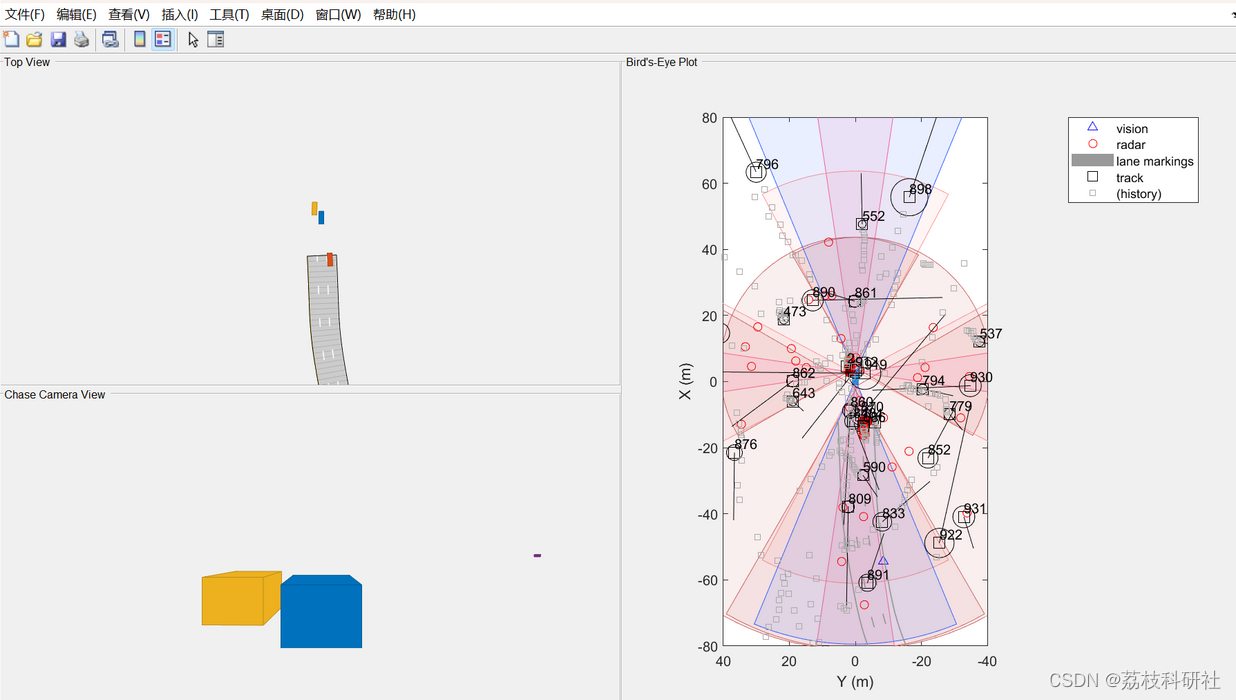
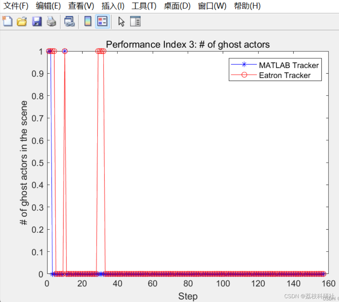
本文使用MATLAB的场景生成器工具箱，通过合成雷达和视觉观察创建一个简单的高速公路驾驶场景。扩展卡尔曼滤波器已被实现以将车辆的状态传播到未来。将投影状态值与当前测量值进行比较以执行跟踪。

一、引言

雷达和视觉传感器是两种常用的目标检测传感器。雷达传感器能够提供目标的距离、方位角和速度信息，而视觉传感器能够提供目标的图像信息。将雷达和视觉数据融合起来，可以提高目标检测的精度和鲁棒性，这对于自动驾驶、智能交通等领域具有重要意义。

二、研究背景与意义

目标级传感器融合是指将来自不同传感器的目标级数据进行融合，以获取更全面、准确的目标信息。雷达和视觉传感器的数据融合可以充分发挥各自的优势，提高目标检测和跟踪的性能。这种融合技术在军事、安防、自动驾驶等领域具有广泛的应用前景。

三、融合方法与技术

数据预处理：对雷达和视觉传感器的数据进行预处理，包括去噪、滤波、校准等操作，以提高数据质量和一致性。
特征提取：从雷达和视觉数据中提取目标的特征，如目标的位置、速度、大小、形状等。
数据关联：将雷达和视觉数据进行关联，即将雷达和视觉传感器所观测到的同一目标进行匹配，以建立目标的对应关系。
融合算法：常见的融合算法包括综合平均法、贝叶斯估计法、D-S法、神经网络法、卡尔曼滤波法等。其中，卡尔曼滤波法及其扩展形式（如扩展卡尔曼滤波EKF）在目标状态估计中得到了广泛应用。
- 综合平均法：把各传感器数据求平均，乘上权重系数。
- 贝叶斯估计法：通过先验信息和样本信息得到后验分布，再对目标进行预测。
- D-S法：采用概率区间和不确定区间判定多证据体下假设的似然函数进行推理。
- 神经网络法：以测量目标的各种参数集为神经网络的输入，输出推荐的目标特征或权重。
目标跟踪与识别：基于融合后的数据，使用跟踪算法对目标进行连续跟踪，并使用识别算法对目标进行分类和识别。

四、研究内容与实现

研究内容：
- 探索雷达和视觉数据的融合方法，提高目标检测和跟踪的准确性和鲁棒性。
- 研究融合算法在自动驾驶、智能交通等领域的应用效果。
实现方法：
- 在MATLAB等仿真环境中，使用MDPDA算法、EKF等算法实现雷达和视觉数据的融合。
- 通过定义传感器配置和使用场景生成器工具箱来合成雷达和视觉观察数据。
- 使用跟踪算法对融合后的数据进行目标跟踪，并使用识别算法对目标进行分类和识别。

五、仿真实验与结果分析

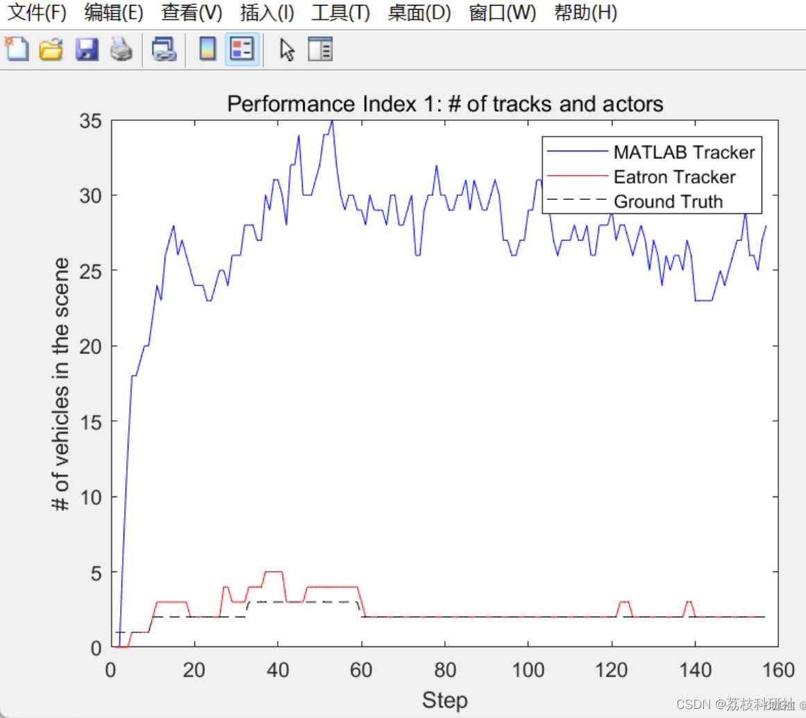
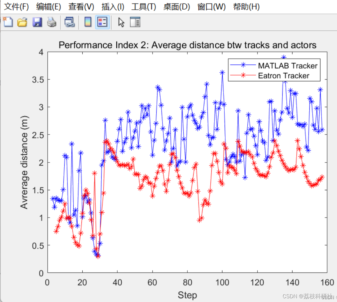
仿真实验设计：设计不同的仿真场景，包括简单场景和复杂场景，以验证融合算法的有效性和鲁棒性。
结果分析：对仿真实验结果进行分析，比较不同融合算法的性能差异，评估融合算法在目标检测和跟踪方面的优势。

六、结论与展望

结论：总结研究成果，指出雷达和视觉合成数据的目标级传感器融合在提高目标检测和跟踪性能方面的有效性和优势。
展望：提出进一步的研究方向，如优化融合算法、提高融合效率、拓展应用领域等。

📚2 运行结果

部分代码：

clear all
close all
clc

%% Parameters

% Assignment gate value
AssignmentThreshold = 30; % The higher the Gate value, the higher the likelihood that every track...
% will be assigned a detection.

% M/N initiation parameters
% The track is "confirmed" if after N consecutive updates at
% least M measurements are assigned to the track after the track initiation.
N = 5;
M = 4;

% Elimination threshold: The track will be deleted after EliminationTH # of updates without
% any measurement update
EliminationTH = 10; % updates

% Measurement Noise
R = [22.1 0 0 0
0 2209 0 0
0 0 22.1 0
0 0 0 2209];

% Process noise
Q= 7e-1.*eye(4);

% Performance anlysis parameters:
XScene = 80;
YScene = 40;
% PerfRadius is defined after scenario generation

%% Generate the Scenario

% Define an empty scenario.
scenario = drivingScenario;
scenario.SampleTime = 0.01; % seconds
SensorsSampleRate = 0.1; % seconds

EgoSpeed = 25; % m/s

%% Simple Scenario (Choice #1)

% Load scenario road and extract waypoints for each lane
Scenario = load('SimpleScenario.mat');
WPs{1} = Scenario.data.ActorSpecifications(2).Waypoints;
WPs{2} = Scenario.data.ActorSpecifications(1).Waypoints;
WPs{3} = Scenario.data.ActorSpecifications(3).Waypoints;

road(scenario, WPs{2}, 'lanes',lanespec(3));

% Ego vehicle (lane 2)
egoCar = vehicle(scenario, 'ClassID', 1);
egoWPs = circshift(WPs{2},-8);
path(egoCar, egoWPs, EgoSpeed);

% Car1 (passing car in lane 3)
Car1 = vehicle(scenario, 'ClassID', 1);
Car1WPs = circshift(WPs{1},0);
path(Car1, Car1WPs, EgoSpeed + 5);

% Car2 (car in lane 1)
Car2 = vehicle(scenario, 'ClassID', 1);
Car2WPs = circshift(WPs{3},-15);
path(Car2, Car2WPs, EgoSpeed -5);

% Ego follower (lane 2)
Car3 = vehicle(scenario, 'ClassID', 1);
Car3WPs = circshift(WPs{2},+5);
path(Car3, Car3WPs, EgoSpeed);

% Car4 (stopped car in lane 1)
Car4 = vehicle(scenario, 'ClassID', 1);
Car4WPs = circshift(WPs{3},-13);
path(Car4, Car4WPs, 1);

ActorRadius = norm([Car1.Length,Car1.Width]);
%---------------------------------------------------------------------------------------------
%% Waypoint generation (Choice #2)

% % Load scenario road and extract waypoints for each lane
% WPs = GetLanesWPs('Scenario3.mat');
% % Define road wtr the middle lane waypoints
% road(scenario, WPs{2}, 'lanes',lanespec(3));
% %%%%%%%%%%%% BE CAREFUL OF LANESPACE(3) %%%%%%%%%%%%%%%%%%%%%%%%%%%%%%%%%%%%%
% % Ego vehicle (lane 2)
% egoCar = vehicle(scenario, 'ClassID', 1);
% path(egoCar, WPs{2}, EgoSpeed); % On right lane
%
% % Car1 (passing car in lane 3)
% Car1 = vehicle(scenario, 'ClassID', 1);
% WPs{1} = circshift(WPs{1},20);
% path(Car1, WPs{1}, EgoSpeed + 2);
%
% % Car2 (slower car in lane 1)
% Car2 = vehicle(scenario, 'ClassID', 1);
% WPs{3} = circshift(WPs{3},-50);
% path(Car2, WPs{3}, EgoSpeed -5);

%---------------------------------------------------------------------------------------------

%% Create a Tracker
% Create a |<matlab:doc('multiObjectTracker') multiObjectTracker>| to track
% the vehicles that are close to the ego vehicle. The tracker uses the
% |initSimDemoFilter| supporting function to initialize a constant velocity
% linear Kalman filter that works with position and velocity.
%
% Tracking is done in 2-D. Although the sensors return measurements in 3-D,
% the motion itself is confined to the horizontal plane, so there is no
% need to track the height.
tracker = multiObjectTracker('FilterInitializationFcn', @initSimDemoFilter, ...
'AssignmentThreshold', 30, 'ConfirmationParameters', [4 5]);
positionSelector = [1 0 0 0; 0 0 1 0]; % Position selector
velocitySelector = [0 1 0 0; 0 0 0 1]; % Velocity selector

%% Define Sensors and Bird's Eye Plot
sensors = SensorsConfig(egoCar,SensorsSampleRate);

BEP = createDemoDisplay(egoCar, sensors);
BEP1 = createDemoDisplay(egoCar, sensors);

%% Fusion Loop for the scenario

Tracks = [];
count = 0;
toSnap = true;
TrackerStep = 0;
time0 = 0;
currentStep = 0;
Performance.Actors.Ground = [];
Performance.Actors.EATracks = [];
Performance.Actors.MATracks = [];
Performance.MeanDistance.EA = [];
Performance.MeanDistance.MA = [];
Performance.GhostActors.EA = [];
Performance.GhostActors.MA = [];
while advance(scenario) %&& ishghandle(BEP.Parent)
currentStep = currentStep + 1;
% Get the scenario time
time = scenario.SimulationTime;

% Get the position of the other vehicle in ego vehicle coordinates
ta = targetPoses(egoCar);

% Simulate the sensors
detections = {};
isValidTime = false(1,length(sensors));
for i = 1:length(sensors)
[sensorDets,numValidDets,isValidTime(i)] = sensors{i}(ta, time);
if numValidDets
for j = 1:numValidDets
% Vision detections do not report SNR. The tracker requires
% that they have the same object attributes as the radar
% detections. This adds the SNR object attribute to vision
% detections and sets it to a NaN.
if ~isfield(sensorDets{j}.ObjectAttributes{1}, 'SNR')
sensorDets{j}.ObjectAttributes{1}.SNR = NaN;
end
end
detections = [detections; sensorDets]; %#ok<AGROW>
end
end

% Update the tracker if there are new detections
if any(isValidTime)
TrackerStep = TrackerStep + 1;