二分类结局变量Logistic回归临床模型预测（二）——基线特征及三线表绘制（一）

 

 本节讲的是二分类结局变量的临床模型预测，与之前讲的Cox回归不同，https://lijingxian19961016.blog.csdn.net/article/details/124088364https://lijingxian19961016.blog.csdn.net/article/details/124088364https://lijingxian19961016.blog.csdn.net/article/details/130053191https://lijingxian19961016.blog.csdn.net/article/details/130053191

二分类结局变量只有发生和不发生，而不考虑时间等协变量。本期的内容主要有以下几节：

1. 介绍

2. 基线特征

3. 单因素多因素logistic回归分析及三线表

4. 构建临床列线图模型

5. 模型评价

6. 外部数据集验证

7. 另一种发文章的办法，分训练集和测试集，分析上述3-6节的内容

下面讲一下基线特征如何做，有两种办法，今天先将第一种比较笨的办法：

先读取数据：

setwd("D:\\Logistic回归临床模型预测")
dir()
data <- read.csv("data——分析.csv",header = T,sep = ",")
head(data)

# #> head(data)
#梗阻 年龄 胃管 进食水时间.天. 身高 体重  BMI 有无吸烟 高血压 糖尿病 心血管疾病 腹部手术史 手术方式
#1   无   54    0              4  160   68 26.6       No     No     No         No         No     腔镜
#2   无   61    0              2  175   89 29.1       No     No    Yes         No         No     腔镜
#3   无   62    0              3  170   80 27.7       No    Yes     No         No         No     腔镜
#4   无   85    0              3  165   60 22.0       No    Yes     No         No         No     腔镜
#5   无   85    0              2  170   80 27.7       No     No     No         No         No     腔镜
#6   无   73    0              1  158   69 27.6       No    Yes     No        Yes        Yes     腔镜

这里我们不看身高和体重，只看BMI，先将年龄和BMI两个连续性变量改成分类变量：

data$年龄 <- ifelse(data$年龄>60,">60","<=60")
data$BMI <- ifelse(data$BMI>24,">24","<=24")
head(data)


#> head(data)
#  梗阻 年龄 胃管 进食水时间.天. 身高 体重  BMI 有无吸烟 高血压 糖尿病 心血管疾病 腹部手术史 手术方式
#1   无 <=60    0              4  160   68  >24       No     No     No         No         No     腔镜
#2   无  >60    0              2  175   89  >24       No     No    Yes         No         No     腔镜
#3   无  >60    0              3  170   80  >24       No    Yes     No         No         No     腔镜
#4   无  >60    0              3  165   60 <=24       No    Yes     No         No         No     腔镜
#5   无  >60    0              2  170   80  >24       No     No     No         No         No     腔镜
#6   无  >60    0              1  158   69  >24       No    Yes     No        Yes        Yes     腔镜

然后使用table函数看不同临床指标在梗阻和不梗阻的患者中的分布情况：

table(data$BMI,data$梗阻)

#> table(data$BMI,data$梗阻)
      
#       无 有
#  <=24 26 13
#  >24  44 12

这里我们需要卡方检验和Fisher检验来观察不同临床指标在有无肠梗阻患者上的分布：

a <- table(data$BMI,data$梗阻)
chisq.test(a)


# > chisq.test(a)

#	Pearson's Chi-squared test with Yates' continuity correction

#data:  a
#X-squared = 1.1224, df = 1, p-value = 0.2894


fisher.test(a)

# > fisher.test(a)

#	Fisher's Exact Test for Count Data

#data:  a
#p-value = 0.239
#alternative hypothesis: true odds ratio is not equal to 1
#95 percent confidence interval:
# 0.1956891 1.5222276
#sample estimates:
#odds ratio 
# 0.5490433 

当配对四个表中有数值小于5，建议用Fisher检验，否则用卡方检验。

还有只要卡方检验不报warning，我们就用卡方检验就行，这里我们讲数据输入到Excel表中，有用的数据如下：

 

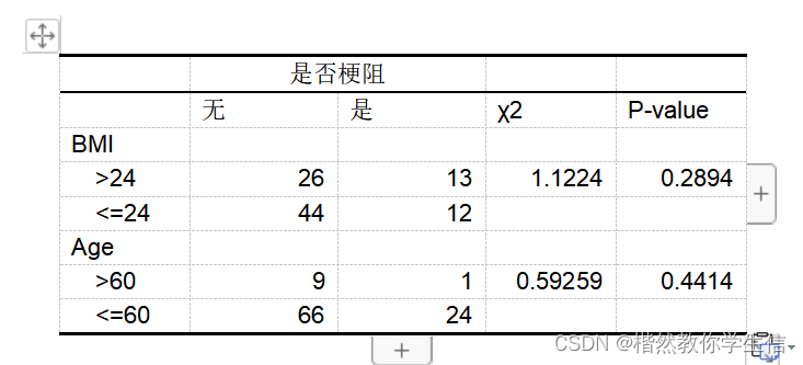
卡方值和p-value，还有患者不同分组的数量，输入到Excel表中：

 

 子类（>24，和<=24）空两格，字体改成Arial格式比较好看，发英文的就把中文改成英文的就行，注意卡方的写法，文章中用的是特殊字符“ χ2” 。

 依次类推，做下一个指标：

 

table(data$年龄,data$梗阻)

a <- table(data$年龄,data$梗阻)
chisq.test(a)

# > chisq.test(a)

#	Pearson's Chi-squared test with Yates' continuity correction

#data:  a
#X-squared = 0.59259, df = 1, p-value = 0.4414

#Warning message:
#In chisq.test(a) : Chi-squared近似算法有可能不准

这里报了warning，说明用卡方可能不准，那么就可以换成 fisher 检验。

fisher.test(a)

# > fisher.test(a)

#	Fisher's Exact Test for Count Data

#data:  a
#p-value = 0.4439
#alternative hypothesis: true odds ratio is not equal to 1
#95 percent confidence interval:
#   0.4103139 149.2394515
#sample estimates:
#odds ratio 
#  3.243412 

 但是这里涉及到要用卡方值的问题，所以没办法用Fisher，不过可以不要卡方值这一项，然后用Fisher的P值。

这里我们依旧用卡方检验的结果吧，将结果输入到excel表中，如下所示：

 依次做完以后，将数据粘贴到word文档，添加上下框线，制成三线表，然后另存为成PDF格式：

 

 下一节讲一个比较简单快速的绘制三线表的方法。