A Riemannian Network for SPD Matrix Learning

weixin_49241211

已于 2023-05-18 07:18:05 修改

阅读量348

点赞数

文章标签： python 开发语言

于 2023-05-18 05:19:20 首次发布

本文链接：https://blog.csdn.net/weixin_49241211/article/details/130734804

版权

Abstract

Symmetric Positive Deﬁnite (SPD) matrix learning methods have become popular in many image and video processing tasks, thanks to their ability to learn appropriate statistical representations while respecting Riemannian geometry of underlying SPD manifolds. In this paper we build a Riemannian network architecture to open up a new direction of SPD matrix non-linear learning in a deep model. In particular, we devise bilinear mapping layers to transform input SPD matrices to more desirable SPD matrices, exploit eigenvalue rectiﬁcation layers to apply a non-linear activation function to the new SPD matrices, and design an eigenvalue logarithm layer to perform Riemannian computing on the resulting SPD matrices for regular output layers. For training the proposed deep network, we exploit a new backpropagation with a variant of stochastic gradient descent on Stiefel manifolds to update the structured connection weights and the involved SPD matrix data. We show through experiments that the proposed SPD matrix network can be simply trained and outperform existing SPD matrix learning and state-of-the-art methods in three typical visual classiﬁcation tasks.

Introduction

Symmetric Positive Deﬁnite (SPD) matrices are often encountered and have made great success in a variety of areas. In medical imaging, they are commonly used in diffusion tensor magnetic resonance imaging (Pennec, Fillard, and Ayache 2006; Arsigny et al. 2007; Jayasumana et al. 2013). In visual recognition, SPD matrix data provide powerful statistical representations for images and videos. Examples include region covariance matrices for pedestrian detection (Tuzel, Porikli, and Meer 2006; Tuzel, Porikli, and Meer 2008; Tosato et al. 2010), joint covariance descriptors for action recognition (Harandi, Salzmann, and Hartley 2014), image set covariance matrices for face recognition (Wang et al. 2012; Huang et al. 2014; Huang et al. 2015b) and second-order pooling for object classiﬁcation (Ionescu, Vantzos, and Sminchisescu 2015).

As a consequence, there has been a growing need to carry out effective computations to interpolate, restore, and classify SPD matrices. However, the computations on SPD matrices often accompany with the challenge of their nonEuclidean data structure that underlies a Riemannian manifold (Pennec, Fillard, and Ayache 2006; Arsigny et al. 2007). Applying Euclidean geometry to SPD matrices directly often results in undesirable effects, such as the swelling of diffusion tensors (Pennec, Fillard, and Ayache 2006). To address this problem, (Pennec, Fillard, and Ayache 2006; Arsigny et al. 2007; Sra 2011) introduced Riemannian metrics, e.g., Log-Euclidean metric (Arsigny et al. 2007), to encode Riemannian geometry of SPD manifolds properly.

By employing these well-studied Riemannian metrics, existing SPD matrix learning approaches typically ﬂatten SPD manifolds via tangent space approximation (Tuzel, Porikli, and Meer 2008; Tosato et al. 2010; Carreira et al. 2012; Fathy, Alavi, and Chellappa 2016), or map them into reproducing kernel Hilbert spaces (Harandi et al. 2012; Wang et al. 2012; Sanin et al. 2013; Quang, Biagio, and Murino 2014; Faraki, Harandi, and Porikli 2015; Zhang et al. 2015). To more faithfully respect the original Riemannian geometry, recent methods (Harandi, Salzmann, and Hartley 2014; Huang et al. 2015b) adopt a geometry-aware SPD matrix learning scheme to pursue a mapping from the original SPD manifold to another one with the same SPD structure. However, all the existing methods merely apply shallow learning, with which traditional methods are typically surpassed by recent popular deep learning methods in many contexts in artiﬁcial intelligence and visual recognition.

In the light of the successful paradigm of deep neural networks (e.g., (LeCun et al. 1998; Krizhevsky, Sutskever, and Hinton 2012)) to perform non-linear computations with effective backpropagation training algorithms, we devise a deep neural network architecture, that receives SPD matrices as inputs and preserves the SPD structure across layers, for SPD matrix non-linear learning. In other words, we aim to design a deep learning architecture to non-linearly learn desirable SPD matrices on Riemannian manifolds. In summary, this paper mainly brings three innovations:

A novel Riemannian network architecture is introduced to open a new direction of SPD matrix deep non-linear learning on Riemannian manifolds.

This work offers a paradigm of incorporating the Riemannian structures into deep network architectures for compressing both of the data space and the weight space.

A new backpropagation is derived to train the proposed network with exploiting a stochastic gradient descent optimization algorithm on Stiefel manifolds.

Related Work

Deep neural networks have exhibited their great powers when the processed data own a Euclidean data structure. In many contexts, however, one may be faced with data deﬁned in non-Euclidean domains. To tackle graph-structured data, (Bruna et al. 2014) presented a spectral formulation of convolutional networks by exploiting a notion of non shiftinvariant convolution that depends on the analogy between the classical Fourier transform and the Laplace-Beltrami eigenbasis. Following (Bruna et al. 2014), a localized spectral network was proposed in (Boscaini et al. 2015) to nonEuclidean domains by generalizing the windowed Fourier transform to manifolds to extract the local behavior of some dense intrinsic descriptor. Similarly, (Masci et al. 2015) proposed a ‘geodesic convolution’ on non-Euclidean local geodesic system of coordinates to extract ‘local patches’ on shape manifolds. The convolutions in this approach were performed by sliding a window over the shape manifolds.

Stochastic gradient descent (SGD) has been the workhorse for optimizing deep neural networks. As an application of the chain rule, backpropagation is commonly employed to compute Euclidean gradients of objective functions, which is the key operation of SGD. Recently, the two works (Ionescu, Vantzos, and Sminchisescu 2015; Gao, Guo, and Wang 2016) extended backpropagation directly on matrices. For example, (Ionescu, Vantzos, and Sminchisescu 2015) formulated matrix backpropagation as a generalized chain rule mechanism for computing derivatives of composed matrix functions with respect to matrix inputs. Besides, the other family of network optimization algorithms exploits Riemannian gradients to handle weight space symmetries in neural networks. For instance, recent works (Bottou 2010; Bonnabel 2013; Ollivier 2013; Marceau-Caron and Ollivier 2016) developed several optimization algorithms by building Riemannian metrics on the activity and parameter space of neural networks, treated as Riemannian manifolds.

Riemannian SPD Matrix Network

Analogously to the well-known convolutional network (ConvNet), the proposed SPD matrix network (SPDNet) also designs fully connected convolution-like layers and rectiﬁed linear units (ReLU)-like layers, named bilinear mapping (BiMap) layers and eigenvalue rectiﬁcation (ReEig) layers respectively. In particular, following the classical manifold learning theory that learning or even preserving the original data structure can beneﬁt classiﬁcation, the BiMap layers are designed to transform the input SPD matrices, that are usually covariance matrices derived from the data, to new SPD matrices with a bilinear mapping. As the classical ReLU layers, the proposed ReEig layers introduce a non-linearity to the SPDNet by rectifying the resulting SPD matrices with a non-linear function. Since SPD matrices reside on non-Euclidean manifolds, we have to devise an eigenvalue logarithm (LogEig) layer to carry out Riemannian computing on them to output their Euclidean forms for any regular output layers. The proposed Riemannian network is conceptually illustrated in Fig.1.

BiMap Layer

The primary function of the SPDNet is to generate more compact and discriminative SPD matrices. To this end, we design the BiMap layer to transform the input SPD matrices to new SPD matrices by a bilinear mapping $f_{b}$ as

$\mathbf{X}_{k}=f_{b}^{(k)}(\mathbf{X}_{k-1};\mathbf{W}_{k})=\mathbf{W}_{k}\mathbf{X}_{k-1}\mathbf{W}_{k}^{T},\quad(1)$

where $X_{k-1}\in S y m_{d_{k-1}}^{+},$ is the input SPD matrix of the k-th layer, $\boldsymbol{W}_k\in\mathbb{R}_*^{d_k\times d_{k-1}},(d_k<d_{k-1})$ is the transformation matrix (connection weights), $\boldsymbol{X}_k \in \mathbb{R}^{d_k \times d_k}$ is the resulting matrix. Note that multiple bilinear mappings can be also performed on each input. To ensure the output ${X}_k$ becomes a valid SPD matrix, the transformation matrix ${W}_k$ is basically required to be a row full-rank matrix. By applying the BiMap layer, the inputs on the original SPD manifold $Sym_{d_{k-1}}^+$ are transformed to new ones which form another SPD manifold $Sym_{d_{k}}^+$ . In other words, the data space on each BiMap layer corresponds to one SPD manifold.

Since the weight space $R_{*}^{d_{k}\times d_{k-1}}$ of full-rank matrices is a non-compact Stiefel manifold where the distance function has no upper bound, directly optimizing on the manifold is infeasible. To handle this problem, one typical solution is to additionally assume the transformation matrix Wk to be orthogonal (semi-orthogonal more exactly here) so that they reside on a compact Stiefel manifold $St(d_k,d_{k-1})$ . As a result, optimizing over the compact Stiefel manifolds can achieve optimal solutions of the transformation matrices.

ReEig Layer

In the context of ConvNets, (Jarrett et al. 2009; Nair and Hinton 2010) presented various rectiﬁed linear units (ReLU) (including the max(0, x) non-linearity) to improve discriminative performance. Hence, exploiting ReLU-like layers to introduce a non-linearity to the context of the SPDNet is also necessary. Inspired by the idea of the max(0, x) nonlinearity, we devise a non-linear function $f_r$ for the ReEig ( $k$ -th) layer to rectify the SPD matrices by tuning up their small positive eigenvalues:

$\boldsymbol{X}_k=f^{(k)}_r(\boldsymbol{X}_{k-1})=\boldsymbol{U}_{k-1}\max(\epsilon\boldsymbol{I},\boldsymbol{\Sigma}_{k-1})U^{T}_{k-1},\quad(2)$

where $U_{k-1}$ and $\boldsymbol{\Sigma}_{k-1}$ are achieved by eigenvalue decomposition (EIG) $\boldsymbol{X}_{k-1}=\boldsymbol{U}_{k-1}\boldsymbol{\Sigma}_{k-1}\boldsymbol{U}_{k-1}^T$ , $\epsilon\$ is a rectiﬁcation threshold, $I$ is an identity matrix, max( $\epsilon\boldsymbol{I},\boldsymbol{\Sigma}_{k-1}$ ) is a diagonal matrix $A$ with diagonal elements being deﬁned as

$\boldsymbol{A}(i,i)=\begin{cases}\boldsymbol{\Sigma}_{k-1}(i,i),&\boldsymbol{\Sigma}_{k-1}(i,i)>\epsilon,\\ \epsilon,&\boldsymbol{\Sigma}_{k-1}(i,i)\leq\epsilon.\end{cases}\quad(3)$

Intuitively, Eqn.2 prevents the input SPD matrices from being close to non-positive ones (while the ReLU yields sparsity). Nevertheless, it is not originally designed for regularization because the inputs are already non-singular after applying BiMap layers. In other words, we always set $\epsilon$ above the top-n smallest eigenvalue even when the eigenvalues of original SPD matrices are all much greater than zero.

Besides, there also exist other feasible strategies to derive a non-linearity on the input SPD matrices. For example, the sigmoidal function (Cybenko 1989) could be considered to extend Eqn.2 to a different activation function. Due to the space limitation, we do not discuss this any further.

Figure 1: Conceptual illustration of the proposed SPD matrix network (SPDNet) architecture.

LogEig Layer

The LogEig layer is designed to perform Riemannian computing on the resulting SPD matrices for output layers with objective functions. As studied in (Arsigny et al. 2007), the Log-Euclidean Riemannian metric is able to endow the Riemannian manifold of SPD matrices with a Lie group structure so that the manifold is reduced to a ﬂat space with the matrix logarithm operation log(·) on the SPD matrices. In the ﬂat space, classical Euclidean computations can be applied to the domain of SPD matrix logarithms. Formally, we employ the Riemannian computation (Arsigny et al. 2007) in the $k$ -th layer to deﬁne the involved function $f_l$ as

$\boldsymbol{X}_k=f^{(k)}_l(\boldsymbol{X}_{k-1})=\log(\boldsymbol{X}_{k-1})=\boldsymbol{U}_{k-1}\log(\boldsymbol{\Sigma}_{k-1})\boldsymbol{U}_{k-1}^T,(4)$

where $\boldsymbol{X}_{k-1}~=~\boldsymbol{U}_{k-1}\boldsymbol{\Sigma}_{k-1}\boldsymbol{U}_{k-1}^{T}$ is an EIG operation,log( ${\Sigma}_{k-1}$ ) is the diagonal matrix of eigenvalue logarithms.

For SPD manifolds, the Log-Euclidean Riemannian computation is particularly simple to use and avoids the high expense of other Riemannian computations (Pennec, Fillard, and Ayache 2006; Sra 2011), while preserving favorable theoretical properties. As for other Riemannian computations on SPD manifolds, please refer to (Pennec, Fillard, and Ayache 2006; Sra 2011) for more studies on their properties.

Other Layers

After applying the LogEig layer, the vector forms of the outputs can be fed into classical Euclidean network layers. For example, the Euclidean fully connected (FC) layer could be inserted after the LogEig layer. The dimensionality of the ﬁlters in the FC layer is set to $d_k\times d_{k-1}$ , where $d_k$ and $d_{k-1}$ are the class number and the dimensionality of the vector forms of the input matrices respectively. The ﬁnal output layer for visual recognition tasks could be a softmax layer used in the context of Euclidean networks.

In addition, the pooling layers and the normalization layers are also important to improve regular Euclidean ConvNets. For the SPDNet, the pooling on SPD matrices can be ﬁrst carried out on their matrix logarithms, and then transform them back to SPD matrices by employing the matrix exponential map exp(·) in the Riemannian framework (Pennec, Fillard, and Ayache 2006; Arsigny et al. 2007). Similarly, the normalization procedure on SPD matrices could be ﬁrst to calculate the mean and variance of their matrix logarithms, and then normalize them with their mean and variance as done in (Ioffe and Szegedy 2015).

Riemannian Matrix Backpropagation

The model of the proposed SPDNet can be written as a series of successive function compositions $f=f^{(l)}\circ f^{(l-1)}\dots\circ f^{(1)}$ with a parameter tuple $\boldsymbol{W}=(\boldsymbol{W}_{l},\boldsymbol{W}_{l-1},\ldots,\boldsymbol{W}_{1})$ , where $f^{(k)}$ is the function for the $k$ -th layer, $W_k$ is the weight parameter of the $k$ -th layer and l is the number of layers. The loss of the $k$ a-th layer could be denoted by a function as $L^{(k)}=\ell\circ f^{(l)}\circ\ldots{f^{(k)}},$ , where $\ell$ is the loss function for the ﬁnal output layer.

Training deep networks often uses stochastic gradient descent (SGD) algorithms. The key operation of one classical SGD algorithm is to compute the gradient of the objective function, which is obtained by an application of the chain rule known as backpropagation (backprop). For the kth layer, the gradients of the weight $W_k$ and the data $X_{k-1}$ can be respectively computed by backprop as

$\begin{gathered} \frac{\partial L^{(k)}(\mathbf{X}_{k-1},y)}{\partial\mathbf{W}_{k}} =\frac{\partial L^{(k+1)}(\boldsymbol{X}_{k},y)}{\partial\boldsymbol{X}_{k}}\frac{\partial f^{(k)}(\boldsymbol{X}_{k-1})}{\partial\boldsymbol{W}_{k}},~~(5) \\ \frac{\partial L^{(k)}(\boldsymbol{X}_{k-1},y)}{\partial\boldsymbol{X}_{k-1}} =\frac{\partial L^{(k+1)}(\boldsymbol{X}_{k},y)}{\partial\boldsymbol{X}_{k}}\frac{\partial f^{(k)}(\boldsymbol{X}_{k-1})}{\partial\boldsymbol{X}_{k-1}},~~(6) \end{gathered}$

where $y$ is the output, $\boldsymbol{X}_{k}=f^{(k)}(\boldsymbol{X}_{k-1})$ . Eqn.5 is the gradient for updating $W_k$ , while Eqn.6 is to compute the gradients of the involved data in the layers below. For simplicity, we often replace $\partial L^{(k)}(\mathbf{X}_{k-1},y)$ with $\partial L(k)$ in the sequel.

There exist two key issues for generalizing backprop to the context of the proposed Riemannian network for SPD matrices. The ﬁrst one is updating the weights in the BiMap layers. As we force the weights to be on Stiefel manifolds, merely using Eqn.5 to compute their Euclidean gradients rather than Riemannian gradients in the procedure of backprop cannot yield valid orthogonal weights. While the gradients of the SPD matrices in the BiMap layers can be calculated by Eqn.6 as usual, computing those with EIG decomposition in the layers of ReEig and LogEig has not been well-solved by the traditional backprop. Thus, it is the second key issue for training the proposed network.

To tackle the ﬁrst issue, we propose a new way of updating the weights deﬁned in Eqn.1 for the BiMap layers by exploiting an SGD setting on Stiefel manifolds. The steepest descent direction for the corresponding loss function $L^{(k)}(\boldsymbol{X}_{k-1},y)$ with respect to $W_k$ on the Stiefel manifold is the Riemannian gradient $\tilde{\nabla}L_{\mathbf{W}_k}^{(k)}$ . To obtain it, the normal component of the Euclidean gradient ${\nabla}L_{\mathbf{W}_k}^{(k)}$ is subtracted to generate the tangential component to the Stiefel manifold. Searching along the tangential direction takes the update in the tangent space of the Stiefel manifold. Then, such the update is mapped back to the Stiefel manifold with a retraction operation. For more details about the Stiefel geometry and retraction, readers are referred to (Edelman, Arias, and Smith 1998) and (Absil, Mahony, and Sepulchre 2008) (Page 45-48, 59). Formally, an update of the current weight ${\boldsymbol{W}}_k^t$ on the Stiefel manifold respects the form

$\begin{gathered} \tilde{\nabla}L_{\boldsymbol{W}_{k}^{t}}^{(k)} =\nabla L_{\boldsymbol{W}_{k}^{t}}^{(k)}-\nabla L_{\boldsymbol{W}_{k}^{t}}^{(k)}(\boldsymbol{W}_{k}^{t})^{T}\boldsymbol{W}_{k}^{t}, (7) \\ \mathbf{W}_k^{t+1} =\Gamma(\mathbf{W}_k^t-\lambda\tilde{\nabla}L_{\mathbf{W}_k^t}^{(k)}), (8) \end{gathered}$

where $\Gamma$ is the retraction operation, $\lambda$ is the learning rate, $\nabla L_{W_k}^{(k)}(\mathbf{W}_k^t)^T\mathbf{W}_k^t$ is the normal component of the Euclidean gradient that can be computed by using Eqn.5 as

$\nabla L_{\mathbf{W}_k^t}^{(k)}=2\frac{\partial L^{(k+1)}}{\partial\mathbf{X}_k}\mathbf{W}_k^t\mathbf{X}_{k-1}.\quad(9)$

As for the second issue, we exploit the matrix generalization of backprop studied in (Ionescu, Vantzos, and Sminchisescu 2015) to compute the gradients of the involved SPD matrices in the ReEig and LogEig layers. In particular, let $\mathcal{F}$ be a function describing the variations of the upper layer variables with respect to the lower layer variables, i.e., $d{\boldsymbol{X}}_{k}=\mathcal{F}(d\boldsymbol{X}_{k-1})$ . With the function $\mathcal{F}$ , a new version of the chain rule Eqn.6 for the matrix backprop is deﬁned as

$\frac{\partial L^{(k)}(\mathbf{X}_{k-1},y)}{\partial\mathbf{X}_{k-1}}=\mathcal{F}^*\left(\frac{\partial L^{(k+1)}(\mathbf{X}_k,y)}{\partial\mathbf{X}_k}\right),\quad(10)$

where $\mathcal{F}^*$ is a non-linear adjoint operator of $\mathcal{F}$ , i.e., $B$ : $\begin{aligned} \\ \mathcal{F}(\boldsymbol{C})&& & =\mathcal{F}^*(\boldsymbol{B}):\boldsymbol{C} \end{aligned}$ , the operator : is the matrix inner product with the property $\begin{aligned} & \\ &\boldsymbol{B}:\boldsymbol{C}& =Tr(\boldsymbol{B}^T\boldsymbol{C}) \end{aligned}$ .

Actually, both of the two functions Eqn.2 and Eqn.4 for the ReEig and LogEig layers involve the EIG operation $\boldsymbol{X}_{k-1}=\boldsymbol{U}_{k-1}\boldsymbol{\Sigma}_{k-1}\boldsymbol{U}_{k-1}^T$ (note that, to increase the readability, we drop the layer indexes for $U_{k-1}$ and $\sum _{k-1}$ in the sequel). Hence, we introduce a virtual layer ( $k^{'}$ layer) for the EIG operation. Applying the new chain rule Eqn.10 and its properties, the update rule for the data $X_{k-1}$ is derived as

$\begin{aligned} &\frac{\partial L^{(k)}}{\partial \boldsymbol{X}_{k-1}} :d\boldsymbol{X}_{k-1} \\ &=\mathcal{F}^*\left(\frac{\partial L^{(k^{'})}}{\partial U}\right):d X_{k-1}+\mathcal{F}^*\left(\frac{\partial L^{(k^{'})}}{\partial\boldsymbol{\Sigma}}\right):d X_{k-1} \\ &=\frac{\partial L^{(k^{'})}}{\partial U}:\mathcal{F}\left(d\mathbf{X}_{k-1}\right)+\frac{\partial L^{(k^{'})}}{\partial\mathbf{\Sigma}}:\mathcal{F}\left(d\mathbf{X}_{k-1}\right) \\ &=\frac{\partial L^{(k')}}{\partial U}:d\boldsymbol U+\frac{\partial L^{(k')}}{\partial\boldsymbol\Sigma}:d\boldsymbol\Sigma, \\ &&\mathrm{(11)} \end{aligned}$

where the two variations $dU$ and $d\sum$ are derived by the variation of the EIG operation $\begin{aligned} & d\boldsymbol{X}_{k-1}= & d\boldsymbol{U}\boldsymbol{\Sigma}\boldsymbol{U}^{T}+ &\end{aligned}\boldsymbol{U}d\boldsymbol{\Sigma}U^T+\boldsymbol{U}\boldsymbol{\Sigma}d\boldsymbol{U}^T$ as:

$\begin{gathered} d\boldsymbol{U} =2\boldsymbol{U}(\boldsymbol{P}^{T}\circ(\boldsymbol{U}^{T}d\boldsymbol{X}_{k-1}\boldsymbol{U})_{s y m}), (12) \\ d\boldsymbol{\Sigma} =(\boldsymbol{U}^T d\boldsymbol{X}_{k-1}\boldsymbol{U})_{diag}, (13) \end{gathered}$

where $\circ$ is the Hadamard product, $\boldsymbol{D}_{sym}=\frac{1}{2}(\boldsymbol{D}+\boldsymbol{D}^T)$ , $\boldsymbol{D}_{diag}$ is $D$ with all off-diagonal elements being 0 (note that we also use these two denotations in the following), $P$ is calculated by operating on the eigenvalues $\sigma$ in $\sum$ :

$\boldsymbol{P}(i,j)=\begin{cases}\frac{1}{\sigma_i-\sigma_j},&i\neq j,\\ 0,&i=j.\end{cases}\quad\text{(14)}$

For more details to derive Eqn.12 and Eqn.13, please refer to (Ionescu, Vantzos, and Sminchisescu 2015). Plugging Eqn.12 and Eqn.13 into Eqn.11 and using the properties of the matrix inner product : can derive the partial derivatives of the loss functions for the ReEig and LogEig layers:

$\begin{aligned} \frac{\partial L^{(k)}}{\partial\boldsymbol{X}_{k-1}}& =2U\left(\boldsymbol{P}^{T}\circ\left(\boldsymbol{U}^{T}\frac{\partial L^{(k^{'})}}{\partial\boldsymbol{U}}\right)_{symm}\right)U^{T} & (15) \\ &+\boldsymbol{U}\left(\frac{\partial L^{(k^{'})}}{\partial\boldsymbol{\Sigma}}\right)_{diag}\boldsymbol{U}^{T}, \end{aligned}$

where $\frac{\partial L^{(k^{'})}}{\partial U}$ and $\frac{\partial L^{(k^{'})}}{\partial\Sigma}$ can be obtained with the same derivation strategy used in Eqn.11. For the function Eqn.2 employed in the ReEig layers, its variation becomes $dX_k=2(d\boldsymbol{U}\operatorname*{max}(\epsilon\boldsymbol{I},\boldsymbol{\Sigma})\boldsymbol{U}^{T})_{s y m}+(\boldsymbol{U}\boldsymbol{Q}d\boldsymbol{\Sigma}\boldsymbol{U}^{T})_{s y m},$ and these two partial derivatives can be computed by

$\begin{gathered} \frac{\partial L^{(k^{'})}}{\partial\boldsymbol{U}} =2\left(\frac{\partial L^{(k+1)}}{\partial\boldsymbol{X}_{k}}\right)_{s y m}\boldsymbol{U}\operatorname*{max}(\boldsymbol{\epsilon}\boldsymbol{I},\boldsymbol{\Sigma}), (16) \\ \frac{\partial L^{(k^{'})}}{\partial\Sigma} =\boldsymbol{QU}^T\left(\frac{\partial L^{(k+1)}}{\partial\boldsymbol{X}_k}\right)_{sym}U, (17) \end{gathered}$

where max( $\epsilon I,\boldsymbol{\Sigma}$ ) is deﬁned in Eqn.3, and Q is the gradient of max( $\epsilon I,\boldsymbol{\Sigma}$ ) with diagonal elements being deﬁned as

$\boldsymbol{Q}(i,i)=\begin{cases}1,&\boldsymbol{\Sigma}(i,i)>\epsilon,\\ 0,&\boldsymbol{\Sigma}(i,i)\leq\epsilon.\end{cases}\quad(18)$

For the function Eqn.4 used in the LogEig layers, its variation is $d\boldsymbol{X}_{k}=2(d\boldsymbol{U}\log{{{(\mathbf{\Sigma})}}}U^{T})_{s y m}+(\boldsymbol{U}\boldsymbol{\Sigma}^{-1}d\boldsymbol{\Sigma}U^{T})_{s y m}.$ . Then we calculate the following two partial derivatives:

$\begin{gathered} \frac{\partial L^{(k^{'})}}{\partial U} =2\left({\frac{\partial L^{(k+1)}}{\partial\mathbf{X}_{k}}}\right)_{s y m}\boldsymbol{U}\log(\boldsymbol{\Sigma}). (19) \\ \frac{\partial L^{(k^{'})}}{\partial\Sigma} =\boldsymbol{\Sigma}^{-1}U^T\left(\frac{\partial L^{(k+1)}}{\partial X_k}\right)_{sym}U, (20) \end{gathered}$

By mainly employing Eqn.7–Eqn.9 and Eqn.15–Eqn.20, the Riemannian matrix backprop for training the SPDNet can be realized. The convergence analysis of the used SGD algorithm on Riemannian manifolds follows the developments in (Bottou 2010; Bonnabel 2013).

Discussion

Although the two works (Harandi, Salzmann, and Hartley 2014; Huang et al. 2015b) have studied the geometry-aware map to preserve SPD structure, our SPDNet exploits more general (i.e., Stiefel manifold) setting for the map, and sets it up in the context of deep learning. Furthermore, we also introduce a non-linearity during learning SPD matrices in the network. Thus, the main theoretical advantage of the proposed SPDNet over the two works is its ability to perform deep learning and non-linear learning mechanisms.

While (Ionescu, Vantzos, and Sminchisescu 2015) introduced a covariance pooling layer into ConvNets starting from images, our SPDNet works on SPD matrices directly and exploits multiple layers tailored for SPD matrix deep learning. From another point of the view, the proposed SPDNet can be built on the top of the network (Ionescu, Vantzos, and Sminchisescu 2015) for deeper SPD matrix learning that starts from images. Moreover, we must claim that our SPDNet is still useful while (Ionescu, Vantzos, and Sminchisescu 2015) will totally break down when the processed data are not covariance matrices for images.

Experiments

We evaluate the proposed SPDNet for three popular visual classiﬁcation tasks including emotion recognition, action recognition and face veriﬁcation, where SPD matrix representations have achieved great successes. The comparing state-of-the-art SPD matrix learning methods are Covariance Discriminative Learning (CDL) (Wang et al. 2012), Log-Euclidean Metric Learning (LEML) (Huang et al. 2015b) and SPD Manifold Learning (SPDML) (Harandi, Salzmann, and Hartley 2014) that uses afﬁne-invariant metric (AIM) (Pennec, Fillard, and Ayache 2006) and stein divergence (Sra 2011). The Riemannian Sparse Representation (RSR) (Harandi et al. 2012) for SPD matrices is also evaluated. Besides, we measure the deep second-order pooling (DeepO2P) network (Ionescu, Vantzos, and Sminchisescu 2015) which introduces a covariance pooling layer into typical ConvNets. For all of them, we use their source codes from authors with tuning their parameters according to the original works. For our SPDNet, we study 4 conﬁgurations, i.e., SPDNet-0BiRe/1BiRe/2BiRe/3BiRe, where iBiRe means using i blocks of BiMap/ReEig. For example, the structure of SPDNet-3BiRe is $X_0\to f_b^{(1)}\to f_r^{(2)}\to f_b^{(3)}\to f_r^{(4)}\to f_b^{(5)}\to f_r^{(6)}\to f_b^{(7)}\to f_s^{(8)}$ aa, where $f_b,f_r,f_l,f_f,f_s$ indicate the BiMap, ReEig, LogEig, FC and softmax log-loss layers respectively. The learning rate λ is ﬁxed as $10^{-2}$ , the batch size is set to 30, the weights are initialized as random semi-orthogonal matrices, and the rectiﬁcation threshold is set to $10^{-4}$ . For training the SPDNet, we just use an i7-2600K (3.40GHz) PC without any GPUs.

Emotion Recognition

We use the popular Acted Facial Expression in Wild (AFEW) (Dhall et al. 2014) dataset for emotion recognition. The AFEW database collects 1,345 videos of facial expressions of actors in movies with close-to-real-world scenarios.

The database is divided into training, validation and test data sets where each video is classiﬁed into one of seven expressions. Since the ground truth of the test set has not been released, we follow (Liu et al. 2014) to report the results on the validation set. To augment the training data, we segment the training videos into 1,747 small clips. For the evaluation, each facial frame is normalized to an image of size 20 × 20. Then, following (Wang et al. 2012), we compute the covariance matrix of size 400 × 400 to represent each video.

On the AFEW database, the dimensionalities of the SPDNet-3BiRe transformation matrices are set to 400 × 200, 200 × 100, 100 × 50 respectively. Training the SPDNet-3BiRe per epoch (500 epoches in total) takes around 2 minutes(m) on this dataset. As show in Table.1, we report the performances of the competing methods including the state-of-the-art method (STM-ExpLet (Liu et al. 2014)) on this database. It shows our proposed SPDNet3BiRe achieves several improvements over the state-of-theart methods although the training data is small.

In addition, we study the behaviors of the proposed SPDNet with different settings. First, we evaluate our SPDNet without using the LogEig layer. Its extremely low accuracy 21.49% shows the layer for Riemannian computing is necessary. Second, we study the case of learning directly on Log-Euclidean forms of original SPD matrices, i.e., SPDNet-0BiRe. The performance of SPDNet-0BiRe is 26.32%, which is clearly outperformed by the deeper SPDNets (e.g., SPDNet-3BiRe). This justiﬁes the importance of using the SPD layers. Besides, SPDNets also clearly outperform DeepO2P that inserts one LogEig-like layer into a standard ConvNet architecture. This somehow validates the improvements are from the contribution of the BiMap and ReEig layers rather than deeper architectures. Third, to study the gains of using multiple BiRe blocks, we compare SPDNet-1BiRe and SPDNet-2BiRe that feed the LogEig layer with SPD matrices of the same size as set in SPDNet-3BiRe. As reported in Table.1, the performance of our SPDNet is improved when stacking more BiRes. Fourth, we also study the power of the designed ReEig layers in Fig.2 (a). The accuracies of the three different rectiﬁcation threshold setting $\epsilon = 10^{-4}$ , $5 \times 10^{-5}$ , 0 are 34.23%, 33.15%, 32.35% respectively, that veriﬁes the success of introducing the non-linearity. Lastly, we also show the convergence behavior of our SPDNet in Fig.2 (b), which suggests it can converge well after hundreds of epoches.

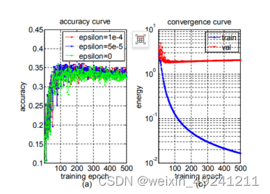
Figure 2: (a) Accuracy curve of the proposed SPDNet-3BiRe at different rectiﬁcation threshold values, and (b) its convergence curve at $\epsilon = 10^{-4}$ for the AFEW dataset.

Action Recognition

We handle the problem of skeleton-based human action recognition using the HDM05 database (Mu¨ller et al. 2007), which is one of the largest-scale datasets for the problem.

On the HDM05 dataset, we conduct 10 random evaluations, in each of which half of sequences are randomly selected for training, and the rest are used for testing. Note that the work (Harandi, Salzmann, and Hartley 2014) only recognizes 14 motion classes while the protocol designed by us is to identify 130 action classes and thus be more challenging. For data augmentation, the training sequences are divided into around 18,000 small sequences in each random evaluation. As done in (Harandi, Salzmann, and Hartley 2014), we represent each sequence by a joint covariance descriptor of size 93 × 93, which is computed by the second order statistics of the 3D coordinates of the 31 joints in each frame.

For our SPDNet-3BiRe, the sizes of the transformation matrices are set to 93 × 70, 70 × 50, 50 × 30 respectively, and its training time at each of 500 epoches is about 4m on average. Table.1 summarizes the results of the comparative algorithms and of the state-of-the-art method (RSRSPDML) (Harandi, Salzmann, and Hartley 2014) on this dataset. As DeepO2P (Ionescu, Vantzos, and Sminchisescu 2015) is merely for image based visual classiﬁcation tasks, we do not evaluate it in the 3D skeleton based action recognition task. We ﬁnd that our SPDNet-3BiRe outperforms the state-of-the-art shallow SPD matrix learning methods by a large margin (more than 13%). This shows that the proposed non-linear deep learning scheme on SPD matrices leads to great improvements when the training data is large enough.

The studies on without using LogEig layers and different conﬁgurations of BiRe blocks are executed as the way of the last evaluation. The performance of the case of without using LogEig layers is 4.89%, again validating the importance of the Riemannian computing layers. Besides, as seen from Table.1, the same conclusions as before for different settings of BiRe blocks can be drew on this database.

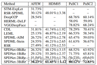
Table 1: The results for the AFEW, HDM05 and PaSC datasets. PaSC1/PaSC2 are the control/handheld testings.

Face Veriﬁcation

For face veriﬁcation, we employ the Point-and-Shoot Challenge (PaSC) database (Beveridge et al. 2013), which is very challenge and widely-used for verifying faces in videos. It includes 1,401 videos taken by control cameras and 1,401 videos captured by handheld cameras for 265 people. In addition, it also contains 280 videos for training.

On the PaSC database, there are control and handheld face veriﬁcation tasks, both of which are to verify a claimed identity in the query video by comparing with the associated target video. As done in (Beveridge, Zhang, and others 2015), we also use the training data (COX) (Huang et al. 2015a) with 900 videos. Similar to the last two experiments, the whole training data are also augmented to 12,529 small video clips. For evaluation, we use the approach of (Parkhiand, Vedaldi, and Zisserman 2015) to extract state-of-theart deep face features on the normalized face images of size 224 × 224. To speed up the training, we employ PCA to ﬁnally get 400-dimensional features. As done in (Huang et al. 2015b), we compute an SPD matrix of size 401 × 401 for each video to fuse its data covariance matrix and mean.

For the evaluation, we conﬁgure the sizes of the SPDNet3BiRe weights to 401 × 200, 200 × 100, 100 × 50 respectively. The time for training the SPDNet-3BiRe at each of 100 epoches is around 15m. Table.1 compares the accuracies of the different methods including the state-of-theart methods (HERML-DeLF (Beveridge, Zhang, and others 2015) and VGGDeepFace (Parkhiand, Vedaldi, and Zisserman 2015)) on the PaSC database. Since the RSR method is designed for recognition tasks rather than veriﬁcation tasks, we do not report its results. Although the used softmax output layer in our SPDNet is not favorable for the veriﬁcation tasks, we ﬁnd that it still achieves the highest performances.

Finally, we can also obtain the same conclusions as before for the studies on different conﬁgurations of the proposed SPDNet as observed from the results on the PaSC dataset.

Conclusio

We proposed a novel deep Riemannian network architecture for opening up a possibility of SPD matrix non-linear learning. To train the SPD network, we exploited a new backpropagation with an SGD setting on Stiefel manifolds. The evaluations on three visual classiﬁcation tasks studied the effectiveness of the proposed network for SPD matrix learning. As future work, we plan to explore more layers, e.g., parallel BiMap layers, pooling layers and normalization layers, to improve the Riemannian network. For further deepening the architecture, we would build the SPD network on the top of existing convolutional networks such as (Ionescu, Vantzos, and Sminchisescu 2015) that start from images. In addition, other interesting directions would be to extend this work for a general Riemannian manifold or to compress traditional network architectures into more compact ones with the proposed SPD or orthogonal constraints.