


、方法1:riskRegression
#Cox校正曲线
#清空
rm(list = ls())
gc()
#导入数据库
library(survival)
data()#查看R包自带数据集
veteran<-veteran#Veterans' Administration Lung Cancer study
str(veteran)#查看数据类型
colnames(veteran)
data<-na.omit(veteran)#清除存在NA的样本
#拆分成测试集和训练集
set.seed(2023)
index<- sample(1:nrow(data),nrow(data)*0.7)
train <- data[index,]
test <- data[-index, ]
dim(train)
dim(test)#42
#校准曲线方法1——riskRegression
library(riskRegression)
#将不同模型绘制在一张图上
fit1 <- coxph(Surv(time, status) ~.,
data = train,
x = T, y = T)
fit2<-coxph(Surv(time, status) ~age+karno,
data = train,
x = T, y = T)
fit3<-coxph(Surv(time, status) ~age+karno+celltype,
data = train,
x = T, y = T)
cox_fit<-Score(list("fit1" = fit1,
"fit2" = fit2,
"fit3" = fit3),
formula = Surv(time, status) ~ 1,
data = test, # 测试集
plots = "calibration",
conf.int = T,
B = 500, #重抽样500次 #交叉验证
M = 40,#抽样样本量 #交叉验证
times=c(100) # 时间
)
plotCalibration(cox_fit,
cens.method="local",
xlab = "Predicted Risk",
ylab = "Observerd RISK",
col=c("red","blue","green"),
legend=F)
legend("topleft",
legend=c("fit1","fit2","fit3"),
fill=c("red","blue","green"))
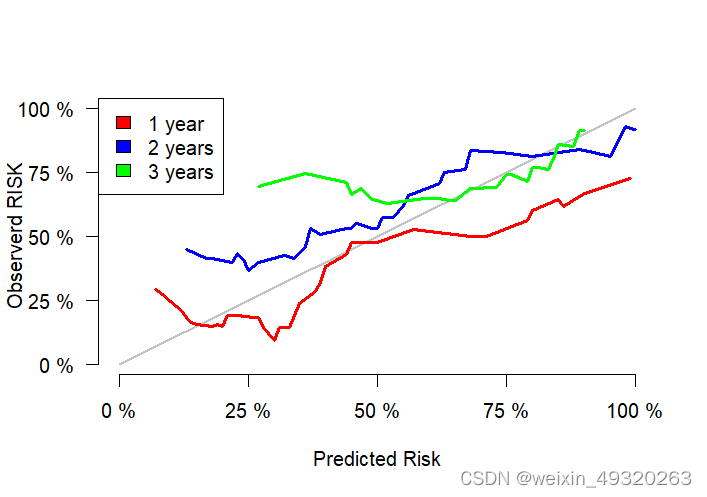
#不同时间点
fit1 <- coxph(Surv(time, status) ~.,
data = train,
x = T, y = T)
cox_fit<-Score(list("fit1" = fit1),
formula = Surv(time, status) ~ 1,
data = test, # 测试集
plots = "calibration",
conf.int = T,
B = 500, #重抽样500次 #交叉验证
M = 40,#抽样样本量 #交叉验证
times=c(50,100,200) # 时间
)
plotCalibration(cox_fit,
times = list(50),
cens.method="local",
xlab = "Predicted Risk",
ylab = "Observerd RISK",
col=list("red"),
legend=F)
plotCalibration(cox_fit,
times = list(100),
cens.method="local",
xlab = "Predicted Risk",
ylab = "Observerd RISK",
col=list("blue"),
add=T,
legend=F)
plotCalibration(cox_fit,
times = list(200),
cens.method="local",
xlab = "Predicted Risk",
ylab = "Observerd RISK",
col=list("green"),
add=T,
legend=F)
legend("topleft",
legend=c("1 year","2 years","3 years"),
fill=c("red","blue","green"))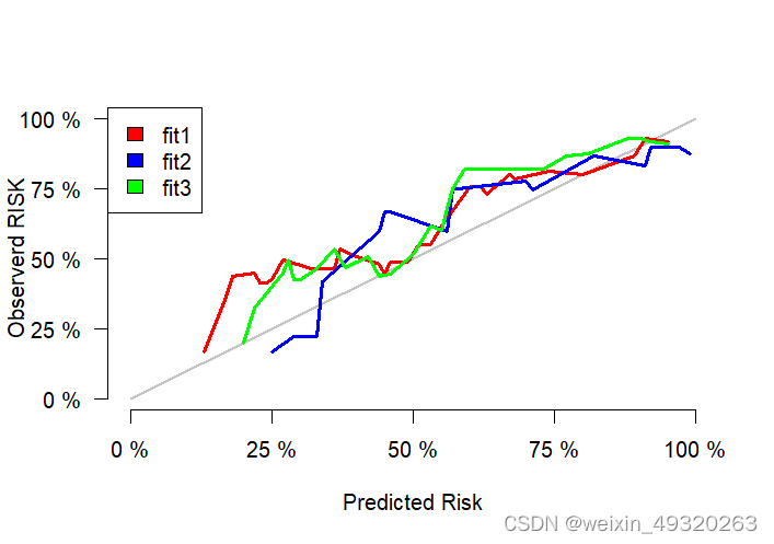
方法2:rms
library(rms)
help(package="rms")
dd <- datadist(veteran)
options(datadist = "dd")
model<-cph(Surv(time,status)~age+karno,
           x=T,y=T,
           surv=T,
           time.inc=100,
           data=train)
calibrate(model,
          u=100,#时间点
          B=30,#抽样数量
          ) %>% plot(xlim=c(0,1),
                     ylim=c(0,1))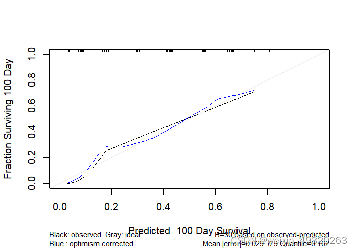


 1655
1655


 被折叠的 条评论
为什么被折叠?
被折叠的 条评论
为什么被折叠?
 到【灌水乐园】发言


