Pytorch3D 入门笔记（二）

如何从初始通用形状的mesh 变形到目标mesh

学习目标：

• How to load a mesh from an .obj file

• How to use the PyTorch3D Meshes datastructure

• How to use 4 different PyTorch3D mesh loss functions

• How to set up an optimization loop

1. Load an obj file and create a Meshes object

3D模型的文件格式是.obj。 用下面的语句加载obj文件。

verts, faces, aux = load_obj(trg_obj)

# verts is a FloatTensor of shape (V, 3) where V is the number of vertices in the mesh

# faces is an object which contains the following LongTensors: verts_idx, normals_idx and textures_idx

faces_idx = faces.verts_idx.to(device)
verts = verts.to(device)

接着标准化（由于我们的目标网格是位于原点、半径为1的球形mesh，因此可以将目标mesh也移动到远点，缩放到大小类似与半径为1的球体）

# We scale normalize and center the target mesh to fit in a sphere of radius 1 centered at (0,0,0).

# (scale, center) will be used to bring the predicted mesh to its original center and scale

# Note that normalizing the target mesh, speeds up the optimization but is not necessary!

center = verts.mean(0)
verts = verts - center
scale = max(verts.abs().max(0)[0])
verts = verts / scale

为目标mesh 创建一个Mesh结构

trg_mesh = Meshes(verts=[verts], faces=[faces_idx])

至此目标mesh就成功导入并创建Mesh对象了。接着初始化通用球形网格。

src_mesh = ico_sphere(4, device)

Visualize the source and target meshes

def plot_pointcloud(mesh, title=""):
    # Sample points uniformly from the surface of the mesh.
    points = sample_points_from_meshes(mesh, 5000)
    x, y, z = points.clone().detach().cpu().squeeze().unbind(1)    
    fig = plt.figure(figsize=(5, 5))
    ax = Axes3D(fig)
    ax.scatter3D(x, z, -y)
    ax.set_xlabel('x')
    ax.set_ylabel('z')
    ax.set_zlabel('y')
    ax.set_title(title)
    ax.view_init(190, 30)
    plt.show()

# %matplotlib notebook
plot_pointcloud(trg_mesh, "Target mesh")
plot_pointcloud(src_mesh, "Source mesh")

2. Optimization loop

利用loss 将source mesh 变换到目标mesh，source mesh 通常可以是一个球面网格。

从球面网格开始，我们学习网格中每个顶点的偏移量，以便在每个优化步骤中预测的网格更接近目标网格。为了实现这一目标，我们最小化:chamfer_distance（表示预测网格与目标网格之间的距离，定义为点云集合之间的倒角距离，这些点云集合是从它们的表面可微采样点产生的。）

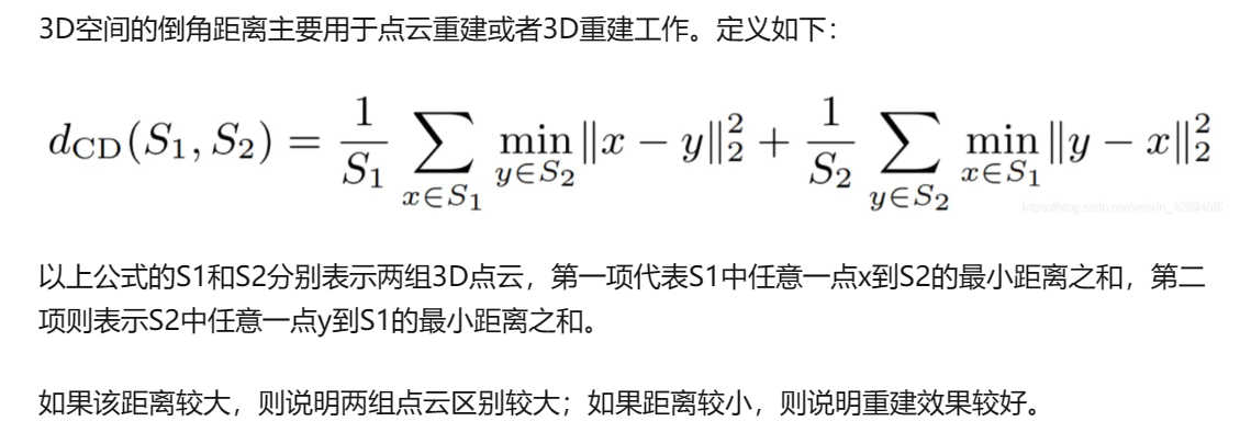
但是仅仅最小化倒角距离将会导致非光滑的形状，因此需要添加形状正则化项来加强平滑性。也就是说，我们添加:

• Mesh _ edge _ length，来限制预测网格中的边长不要过于长。

• mesh_normal_consistency它强化了相邻面的法线的一致性。

• mesh_laplacian_smoothing是拉普拉斯正则化器。

下面是一个标准的优化过程的代码示例。

# We will learn to deform the source mesh by offsetting its vertices
# The shape of the deform parameters is equal to the total number of vertices in src_mesh
deform_verts = torch.full(src_mesh.verts_packed().shape, 0.0, device=device, requires_grad=True)

# The optimizer
optimizer = torch.optim.SGD([deform_verts], lr=1.0, momentum=0.9)

# Number of optimization steps
Niter = 2000
# Weight for the chamfer loss
w_chamfer = 1.0 
# Weight for mesh edge loss
w_edge = 1.0 
# Weight for mesh normal consistency
w_normal = 0.01 
# Weight for mesh laplacian smoothing
w_laplacian = 0.1 
# Plot period for the losses
plot_period = 250
loop = tqdm(range(Niter))

chamfer_losses = []
laplacian_losses = []
edge_losses = []
normal_losses = []

%matplotlib inline

for i in loop:
    # Initialize optimizer
    optimizer.zero_grad()
    
    # Deform the mesh
    new_src_mesh = src_mesh.offset_verts(deform_verts)
    
    # We sample 5k points from the surface of each mesh 
    sample_trg = sample_points_from_meshes(trg_mesh, 5000)
    sample_src = sample_points_from_meshes(new_src_mesh, 5000)
    
    # We compare the two sets of pointclouds by computing (a) the chamfer loss
    loss_chamfer, _ = chamfer_distance(sample_trg, sample_src)
    
    # and (b) the edge length of the predicted mesh
    loss_edge = mesh_edge_loss(new_src_mesh)
    
    # mesh normal consistency
    loss_normal = mesh_normal_consistency(new_src_mesh)
    
    # mesh laplacian smoothing
    loss_laplacian = mesh_laplacian_smoothing(new_src_mesh, method="uniform")
    
    # Weighted sum of the losses
    loss = loss_chamfer * w_chamfer + loss_edge * w_edge + loss_normal * w_normal + loss_laplacian * w_laplacian
    
    # Print the losses
    loop.set_description('total_loss = %.6f' % loss)
    
    # Save the losses for plotting
    chamfer_losses.append(float(loss_chamfer.detach().cpu()))
    edge_losses.append(float(loss_edge.detach().cpu()))
    normal_losses.append(float(loss_normal.detach().cpu()))
    laplacian_losses.append(float(loss_laplacian.detach().cpu()))
    
    # Plot mesh
    if i % plot_period == 0:
        plot_pointcloud(new_src_mesh, title="iter: %d" % i)
        
    # Optimization step
    loss.backward()
    optimizer.step()

3. Visualize the loss

fig = plt.figure(figsize=(13, 5))
ax = fig.gca()
ax.plot(chamfer_losses, label="chamfer loss")
ax.plot(edge_losses, label="edge loss")
ax.plot(normal_losses, label="normal loss")
ax.plot(laplacian_losses, label="laplacian loss")
ax.legend(fontsize="16")
ax.set_xlabel("Iteration", fontsize="16")
ax.set_ylabel("Loss", fontsize="16")
ax.set_title("Loss vs iterations", fontsize="16");

4. Save the predicted mesh

# Fetch the verts and faces of the final predicted mesh
final_verts, final_faces = new_src_mesh.get_mesh_verts_faces(0)

# Scale normalize back to the original target size
final_verts = final_verts * scale + center

# Store the predicted mesh using save_obj
final_obj = os.path.join('./', 'final_model.obj')
save_obj(final_obj, final_verts, final_faces)