


1. 安装CasADi优化库
2. 安装cartpole_casadi_cplusplus库
3. 运行例程
4. 轨迹优化matlab代码解读,例子为质量块最小力
An Introduction to Trajectory Optimization: How to Do Your Own Direct Collocation
文本和代码资料链接https://epubs.siam.org/doi/abs/10.1137/16M1062569
1. 安装CasADi优化库
使用运行机器狗仿真的yobogo的ubuntu16.04系统,这样不用重复安装IPOPT库
安装教程参考InstallationLinux · casadi/casadi Wiki · GitHub
但是需要做一些修改,否则安装不上cmake -DWITH_IPOPT=true ..
安装过程如下,先下载过来,然后编译
git clone https://github.com/casadi/casadi.git -b master casadi

git clone https://github.com/casadi/casadi.git casadi && cd casadi && git checkout 2.0.x

git pull

cd casadi
mkdir build
cd build
cmake编译时不要使用教程上提供的“cmake -DWITH_PYTHON=ON ..”换成如下指令,否则会报can not load shared library "libcasadi_nlpsol_ipopt.so"的错
cmake -DWITH_IPOPT=true ..make
sudo make install
make doc2. 安装cartpole_casadi_cplusplus库
按照给出来的步骤安装
GitHub - ytwboxing/cartpole_casadi_cplusplus: 使用casadi的C++接口写的shooting/collocation轨迹优化示例代码
但是要使用cmake -DWITH_PYTHON=ON .. 代替 cmake ..的指令,如下:
mkdir build && cd build
cmake -DWITH_PYTHON=ON ..
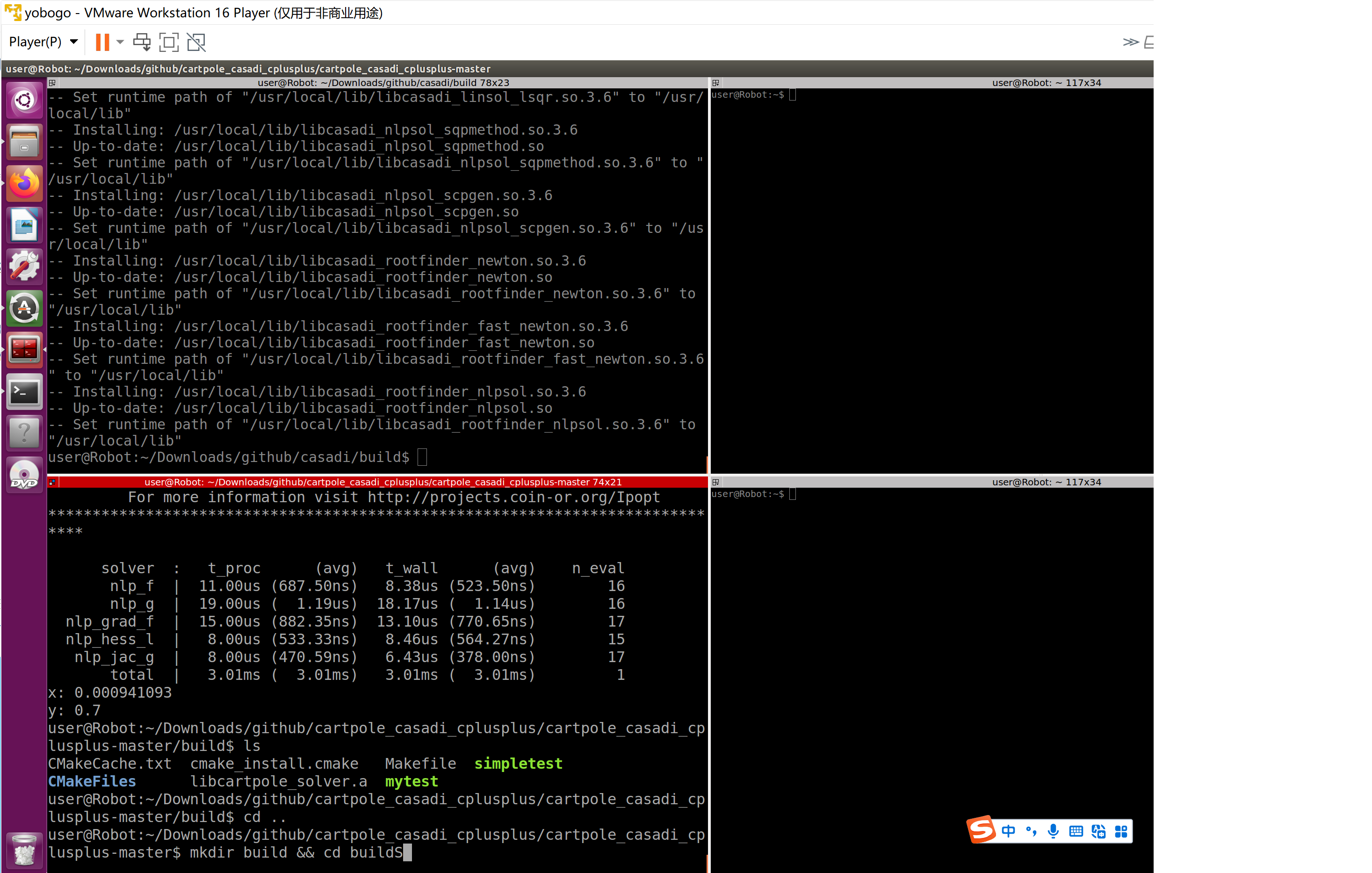
make3. 运行例程
编译成功后运行生成的可执行文件
./mytest相关理论基础见如下文末知乎链接
(附代码)基于casadi C++接口的single/multiple shooting方法轨迹规划示例 - 知乎
可以参考知乎上国外Matthew Kelly的课程资料
本人觉得Underactuated Robotics这个也很好,上面有在线的deepnote代码,方便理解:
Ch. 10 - Trajectory Optimization
4. 轨迹优化matlab代码解读,例子为质量块最小力
配置好问题后,最终调用soln(iter) = hermiteSimpson(P)函数进行求解,hermiteSimpson函数中关键的步骤为soln = directCollocation(problem);directCollocation函数实际上调用了 fmincon 来解决轨迹优化问题。fmincon 函数是用于解决非线性规划(NLP)问题的强大工具。
下面将hermiteSimpson.m和directCollocation.m的代码如下
P = problem
包含以下字段的 struct:
func: [1×1 struct]
bounds: [1×1 struct]
guess: [1×1 struct]
options: [1×1 struct]
fmincon 函数主要是要进行如下的一些配置
P.x0 = zGuess;
zGuess为将每一个网格点的t,x,u按照如下顺序打包成一个向量z = [tSpan;xCol;uCol];
P.lb = zLow;
P.ub = zUpp;
P.Aineq = []; P.bineq = [];
P.Aeq = []; P.beq = [];
P.options = Opt.nlpOpt;
P.solver = 'fmincon';
[zSoln, objVal,exitFlag,output] = fmincon(P);
实现思路如下:
1. hermite即为三次样条曲线,Simpson法用于积分法求曲线长度,每个hermiteSimpson段segment,需要在段中间多加一个点
function soln = hermiteSimpson(problem)
% soln = hermiteSimpson(problem)
%
% This function transcribes a trajectory optimization problem using the
% Hermite-Simpson (Seperated) method for enforcing the dynamics. It can be
% found in chapter four of Bett's book:
%
%   John T. Betts, 2001
%   Practical Methods for Optimal Control Using Nonlinear Programming
%
% For details on the input and output, see the help file for trajOpt.m
%
% Method specific parameters:
%
%   problem.options.method = 'hermiteSimpson'
%   problem.options.hermiteSimpson = struct with method parameters:
%       .nGrid = number of grid points to use for transcription
%
% This transcription method is compatable with analytic gradients. To
% enable this option, set:
%   problem.nlpOpt.GradObj = 'on'
%   problem.nlpOpt.GradConstr = 'on'
%
% Then the user-provided functions must provide gradients. The modified
% function templates are as follows:
%
%         [dx, dxGrad] = dynamics(t,x,u)
%                 dx = [nState, nTime] = dx/dt = derivative of state wrt time
%                 dxGrad = [nState, 1+nx+nu, nTime]
%
%         [dObj, dObjGrad] = pathObj(t,x,u)
%                 dObj = [1, nTime] = integrand from the cost function
%                 dObjGrad = [1+nx+nu, nTime]
%
%         [c, ceq, cGrad, ceqGrad] = pathCst(t,x,u)
%                 c = [nCst, nTime] = column vector of inequality constraints  ( c <= 0 )
%                 ceq = [nCstEq, nTime] = column vector of equality constraints ( c == 0 )
%                 cGrad = [nCst, 1+nx+nu, nTime];
%                 ceqGrad = [nCstEq, 1+nx+nu, nTime];
%
%         [obj, objGrad] = bndObj(t0,x0,tF,xF)
%                 obj = scalar = objective function for boundry points
%                 objGrad = [1+nx+1+nx, 1]
%
%         [c, ceq, cGrad, ceqGrad] = bndCst(t0,x0,tF,xF)
%                 c = [nCst,1] = column vector of inequality constraints  ( c <= 0 )
%                 ceq = [nCstEq,1] = column vector of equality constraints ( c == 0 )
%                 cGrad = [nCst, 1+nx+1+nx];
%                 ceqGrad = [nCstEq, 1+nx+1+nx];
%

% Each segment needs an additional data point in the middle, thus:
nGrid = 2*problem.options.hermiteSimpson.nSegment+1;

% Print out some solver info if desired:
if problem.options.verbose > 0
    fprintf('  -> Transcription via Hermite-Simpson method, nSegment = %d\n',...
        problem.options.hermiteSimpson.nSegment);
end

%%%% Method-specific details to pass along to solver:

%Simpson quadrature for integration of the cost function:
% 辛普森求积法(Simpson quadrature)是一种数值积分方法,
% 它属于牛顿-柯特斯(Newton-Cotes)公式的一种,
% 具体为二阶牛顿-柯特斯闭型积分公式,
% 即通过将函数近似为抛物线来进行积分估算。
% 这种方法相较于一阶的梯形法则(Trapezoidal Rule)能提供更高的精度。
problem.func.weights = (2/3)*ones(nGrid,1);
problem.func.weights(2:2:end) = 4/3;
problem.func.weights([1,end]) = 1/3;
% 权重,起始最小,中间较大且交叉。
    % 0.3333
    % 1.3333
    % 0.6667
    % 1.3333
    % 0.6667
    % 1.3333
    % 0.3333


% Hermite-Simpson calculation of defects:
problem.func.defectCst = @computeDefects;
% 目的是计算沿轨迹的系统连续动力学中的缺陷(defects),
% 以及这些缺陷相对于决策变量的梯度。
% 缺陷通常用于评估一个系统在给定轨迹上是否遵循其动力学方程。
% 如果系统完美遵循其动力学,那么缺陷应该为零。
% x: 状态矩阵,其维度为 [nState, nTime],其中 nState 是状态变量的数量,nTime 是轨迹上的时间点数量。
% 这个矩阵包含了轨迹上每个时间点的状态。
% f: 动力学矩阵,其维度与 x 相同,包含了每个时间点的状态变化率(即动力学)。
% defects: 缺陷矩阵,其维度为 [nState, nTime-1]。这个矩阵包含了轨迹上相邻点之间的动力学误差,即 f(t) * dt - (x(t+1) - x(t))。
% 它衡量了系统在每个时间步上是否严格遵循其动力学。
% 首先,计算每个时间步上的动力学预测值 f(t) * dt,这表示如果系统完全遵循其动力学,则下一个时间点的状态变化量。
% 然后,计算实际状态变化量 x(t+1) - x(t)。
% 接着,将两者相减得到每个时间步上的缺陷 defects。
%%%% The key line - solve the problem by direct collocation:
soln = directCollocation(problem);

% Use method-consistent interpolation
tSoln = soln.grid.time;
xSoln = soln.grid.state;
uSoln = soln.grid.control;
fSoln = problem.func.dynamics(tSoln,xSoln,uSoln);
soln.interp.state = @(t)( pwPoly3(tSoln,xSoln,fSoln,t) );
soln.interp.control = @(t)(pwPoly2(tSoln,uSoln,t));

% Interpolation for checking collocation constraint along trajectory:
%  collocation constraint = (dynamics) - (derivative of state trajectory)
soln.interp.collCst = @(t)( ...
    problem.func.dynamics(t, soln.interp.state(t), soln.interp.control(t))...
    - pwPoly2(tSoln,fSoln,t) );

% Use multi-segment simpson quadrature to estimate the absolute local error
% along the trajectory.
absColErr = @(t)(abs(soln.interp.collCst(t)));
nSegment = problem.options.hermiteSimpson.nSegment;
nState = size(xSoln,1);
nQuadSegment = 5;   %Divide each segment into this many sub-segments
soln.info.error = zeros(nState,nSegment);
for i=1:nSegment
    idx = 2*i + [-1,1];
    soln.info.error(:,i) = simpsonQuadrature(absColErr,tSoln(idx(1)),tSoln(idx(2)),nQuadSegment);
end

end


%%%%~~~~~~~~~~~~~~~~~~~~~~~~~~~~~~~~~~~~~~~~~~~~~~~~~~~~~~~~~~~~~~~~~~~%%%%
%%%%                          SUB FUNCTIONS                            %%%%
%%%%~~~~~~~~~~~~~~~~~~~~~~~~~~~~~~~~~~~~~~~~~~~~~~~~~~~~~~~~~~~~~~~~~~~%%%%


function [defects, defectsGrad] = computeDefects(dt,x,f,dtGrad,xGrad,fGrad)
%
% This function computes the defects that are used to enforce the
% continuous dynamics of the system along the trajectory.
%
% INPUTS:
%   dt = time step (scalar)
%   x = [nState, nTime] = state at each grid-point along the trajectory
%   f = [nState, nTime] = dynamics of the state along the trajectory
%   ~~~~~~~~~~~~~~~~~~~~~~~~~~~~~
%   dtGrad = [2,1] = gradient of time step with respect to [t0; tF]
%   xGrad = [nState,nTime,nDecVar] = gradient of trajectory wrt dec vars
%   fGrad = [nState,nTime,nDecVar] = gradient of dynamics wrt dec vars
%
% OUTPUTS:
%   defects = [nState, nTime-1] = error in dynamics along the trajectory
%   defectsGrad = [nState, nTime-1, nDecVars] = gradient of defects
%

nTime = size(x,2);

iLow = 1:2:(nTime-1);
iMid = iLow + 1;
iUpp = iMid + 1;

xLow = x(:,iLow);
xMid = x(:,iMid);
xUpp = x(:,iUpp);

fLow = f(:,iLow);
fMid = f(:,iMid);
fUpp = f(:,iUpp);

% Mid-point constraint (Hermite)
defectMidpoint = xMid - (xUpp+xLow)/2 - dt*(fLow-fUpp)/4;

% Interval constraint (Simpson)
defectInterval = xUpp - xLow - dt*(fUpp + 4*fMid + fLow)/3;

% Pack up all defects:
defects = [defectMidpoint, defectInterval];


%%%% Gradient Calculations:
if nargout == 2

    xLowGrad = xGrad(:,iLow,:);
    xMidGrad = xGrad(:,iMid,:);
    xUppGrad = xGrad(:,iUpp,:);

    fLowGrad = fGrad(:,iLow,:);
    fMidGrad = fGrad(:,iMid,:);
    fUppGrad = fGrad(:,iUpp,:);

    % Mid-point constraint (Hermite)
    dtGradTerm = zeros(size(xMidGrad));
    dtGradTerm(:,:,1) = -dtGrad(1)*(fLow-fUpp)/4;
    dtGradTerm(:,:,2) = -dtGrad(2)*(fLow-fUpp)/4;
    defectMidpointGrad = xMidGrad - (xUppGrad+xLowGrad)/2 + dtGradTerm + ...
        - dt*(fLowGrad-fUppGrad)/4;

    % Interval constraint (Simpson)
    dtGradTerm = zeros(size(xUppGrad));
    dtGradTerm(:,:,1) = -dtGrad(1)*(fUpp + 4*fMid + fLow)/3;
    dtGradTerm(:,:,2) = -dtGrad(2)*(fUpp + 4*fMid + fLow)/3;
    defectIntervalGrad = xUppGrad - xLowGrad + dtGradTerm + ...
        - dt*(fUppGrad + 4*fMidGrad + fLowGrad)/3;

    %Pack up the gradients of the defects:
    defectsGrad = cat(2,defectMidpointGrad,defectIntervalGrad);

end

end


%%%%%%%%%%%%%%%%%%%%%%%%%%%%%%%%%%%%%%%%%%%%%%%%%%%%%%%%%%%%%%%%%%%%%%%%%%%
%
% Functions for interpolation of the control solution
%

function x = pwPoly2(tGrid,xGrid,t)
% x = pwPoly2(tGrid,xGrid,t)
%
% This function does piece-wise quadratic interpolation of a set of data,
% given the function value at the edges and midpoint of the interval of
% interest.
%
% INPUTS:
%   tGrid = [1, 2*n-1] = time grid, knot idx = 1:2:end
%   xGrid = [m, 2*n-1] = function at each grid point in tGrid
%   t = [1, k] = vector of query times (must be contained within tGrid)
%
% OUTPUTS:
%   x = [m, k] = function value at each query time
%
% NOTES:
%   If t is out of bounds, then all corresponding values for x are replaced
%   with NaN
%

nGrid = length(tGrid);
if mod(nGrid-1,2)~=0 || nGrid < 3
    error('The number of grid-points must be odd and at least 3');
end

% Figure out sizes
n = floor((length(tGrid)-1)/2);
m = size(xGrid,1);
k = length(t);
x = zeros(m, k);

% Figure out which segment each value of t should be on
edges = [-inf, tGrid(1:2:end), inf];
[~, bin] = histc(t,edges);

% Loop over each quadratic segment
for i=1:n
    idx = bin==(i+1);
    if sum(idx) > 0
        gridIdx = 2*(i-1) + [1,2,3];
        x(:,idx) = quadInterp(tGrid(gridIdx),xGrid(:,gridIdx),t(idx));
    end
end

% Replace any out-of-bounds queries with NaN
outOfBounds = bin==1 | bin==(n+2);
x(:,outOfBounds) = nan;

% Check for any points that are exactly on the upper grid point:
if sum(t==tGrid(end))>0
    x(:,t==tGrid(end)) = xGrid(:,end);
end

end


function x = quadInterp(tGrid,xGrid,t)
%
% This function computes the interpolant over a single interval
%
% INPUTS:
%   tGrid = [1, 3] = time grid
%   xGrid = [m, 3] = function grid
%   t = [1, p] = query times, spanned by tGrid
%
% OUTPUTS:
%   x = [m, p] = function at query times
%

% Rescale the query points to be on the domain [-1,1]
t = 2*(t-tGrid(1))/(tGrid(3)-tGrid(1)) - 1;

% Compute the coefficients:
a = 0.5*(xGrid(:,3) + xGrid(:,1)) - xGrid(:,2);
b = 0.5*(xGrid(:,3)-xGrid(:,1));
c = xGrid(:,2);

% Evaluate the polynomial for each dimension of the function:
p = length(t);
m = size(xGrid,1);
x = zeros(m,p);
tt = t.^2;
for i=1:m
    x(i,:) = a(i)*tt + b(i)*t + c(i);
end

end


%%%%%%%%%%%%%%%%%%%%%%%%%%%%%%%%%%%%%%%%%%%%%%%%%%%%%%%%%%%%%%%%%%%%%%%%%%%
%
%  Functions for interpolation of the state solution
%


function x = pwPoly3(tGrid,xGrid,fGrid,t)
% x = pwPoly3(tGrid,xGrid,fGrid,t)
%
% This function does piece-wise quadratic interpolation of a set of data,
% given the function value at the edges and midpoint of the interval of
% interest.
%
% INPUTS:
%   tGrid = [1, 2*n-1] = time grid, knot idx = 1:2:end
%   xGrid = [m, 2*n-1] = function at each grid point in time
%   fGrid = [m, 2*n-1] = derivative at each grid point in time
%   t = [1, k] = vector of query times (must be contained within tGrid)
%
% OUTPUTS:
%   x = [m, k] = function value at each query time
%
% NOTES:
%   If t is out of bounds, then all corresponding values for x are replaced
%   with NaN
%

nGrid = length(tGrid);
if mod(nGrid-1,2)~=0 || nGrid < 3
    error('The number of grid-points must be odd and at least 3');
end

% Figure out sizes
n = floor((length(tGrid)-1)/2);
m = size(xGrid,1);
k = length(t);
x = zeros(m, k);

% Figure out which segment each value of t should be on
edges = [-inf, tGrid(1:2:end), inf];
[~, bin] = histc(t,edges);

% Loop over each quadratic segment
for i=1:n
    idx = bin==(i+1);
    if sum(idx) > 0
        kLow = 2*(i-1) + 1;
        kMid = kLow + 1;
        kUpp = kLow + 2;
        h = tGrid(kUpp)-tGrid(kLow);
        xLow = xGrid(:,kLow);
        fLow = fGrid(:,kLow);
        fMid = fGrid(:,kMid);
        fUpp = fGrid(:,kUpp);
        alpha = t(idx) - tGrid(kLow);
        x(:,idx) = cubicInterp(h,xLow, fLow, fMid, fUpp,alpha);
    end
end

% Replace any out-of-bounds queries with NaN
outOfBounds = bin==1 | bin==(n+2);
x(:,outOfBounds) = nan;

% Check for any points that are exactly on the upper grid point:
if sum(t==tGrid(end))>0
    x(:,t==tGrid(end)) = xGrid(:,end);
end

end


function x = cubicInterp(h,xLow, fLow, fMid, fUpp,del)
%
% This function computes the interpolant over a single interval
%
% INPUTS:
%   h = time step (tUpp-tLow)
%   xLow = function value at tLow
%   fLow = derivative at tLow
%   fMid = derivative at tMid
%   fUpp = derivative at tUpp
%   del = query points on domain [0, h]
%
% OUTPUTS:
%   x = [m, p] = function at query times
%

%%% Fix matrix dimensions for vectorized calculations
nx = length(xLow);
nt = length(del);
xLow = xLow*ones(1,nt);
fLow = fLow*ones(1,nt);
fMid = fMid*ones(1,nt);
fUpp = fUpp*ones(1,nt);
del = ones(nx,1)*del;

a = (2.*(fLow - 2.*fMid + fUpp))./(3.*h.^2);
b = -(3.*fLow - 4.*fMid + fUpp)./(2.*h);
c = fLow;
d = xLow;

x = d + del.*(c + del.*(b + del.*a));

end
directCollocation.m函数,内容如下
function soln = directCollocation(problem)
% soln = directCollocation(problem)
%
% TrajOpt utility function
%
% This function is designed to be called by either "trapezoid" or
% "hermiteSimpson". It actually calls FMINCON to solve the trajectory
% optimization problem.
%
%

%To make code more readable
G = problem.guess;
B = problem.bounds;
F = problem.func;
Opt = problem.options;

nGrid = length(F.weights);

flagGradObj = strcmp(Opt.nlpOpt.GradObj,'on');
flagGradCst = strcmp(Opt.nlpOpt.GradConstr,'on');

% Print out notice about analytic gradients
if Opt.verbose > 0
    if flagGradObj
        fprintf('      - using analytic gradients of objective function\n');
    end
    if flagGradCst
        fprintf('      - using analytic gradients of constraint function\n');
    end
    fprintf('\n');
end

% Interpolate the guess at the grid-points for transcription:
guess.tSpan = G.time([1,end]);
guess.time = linspace(guess.tSpan(1), guess.tSpan(2), nGrid);
guess.state = interp1(G.time', G.state', guess.time')';
guess.control = interp1(G.time', G.control', guess.time')';
% 给定的猜测轨迹(包括时间和状态/控制变量)在新的网格点上进行插值,
% 以便用于后续的转录(即将连续时间问题转换为离散时间问题)和数值优化。
[zGuess, pack] = packDecVar(guess.time, guess.state, guess.control);
% 这个函数的作用是将时间(t)、状态(x)和控制(u)矩阵合并成一个单一的向量。
% 这种操作在轨迹优化和其他需要处理大量变量的数值方法中很常见,
% 它简化了后续的计算和存储过程。
% 首先,函数会确定z向量的长度,这个长度是2 + nTime*(nState+nControl),其中2可能用于额外的信息(尽管这里未明确说明)。
% 然后,函数会按照某种顺序(比如先时间,然后是每个时间点的状态和控制变量)将t、x和u中的数据填充到z向量中。
% 同时,函数会设置pack结构体,以便后续可以将z向量转换回原始的t、x和u矩阵。
if flagGradCst || flagGradObj
    gradInfo = grad_computeInfo(pack);
end

% Unpack all bounds:
tLow = linspace(B.initialTime.low, B.finalTime.low, nGrid);
xLow = [B.initialState.low, B.state.low*ones(1,nGrid-2), B.finalState.low];
uLow = B.control.low*ones(1,nGrid);
zLow = packDecVar(tLow,xLow,uLow);
%每一个网格点的下界

tUpp = linspace(B.initialTime.upp, B.finalTime.upp, nGrid);
xUpp = [B.initialState.upp, B.state.upp*ones(1,nGrid-2), B.finalState.upp];
uUpp = B.control.upp*ones(1,nGrid);
zUpp = packDecVar(tUpp,xUpp,uUpp);
%每一个网格点的上界
%%%% Set up problem for fmincon:

% P.objective是fmincon函数的目标函数
if flagGradObj
    P.objective = @(z)( ...
        myObjGrad(z, pack, F.pathObj, F.bndObj, F.weights, gradInfo) );   %Analytic gradients
    % 该函数的核心功能在于接收一个包含决策变量的列向量z,以及一个包含转换细节的结构体pack。
    % 利用这些信息,函数能够重构出时间、状态和控制变量。
    % 随后,它将这些变量传递给用户自定义的积分目标函数pathObj和终点目标函数endObj,
    % 从而计算出与这组决策变量相对应的总成本(或称为代价、损失等)cost。
else
    P.objective = @(z)( ...
        myObjective(z, pack, F.pathObj, F.bndObj, F.weights) );   %Numerical gradients
end
if flagGradCst
    P.nonlcon = @(z)( ...
        myCstGrad(z, pack, F.dynamics, F.pathCst, F.bndCst, F.defectCst, gradInfo) ); %Analytic gradients
else
    P.nonlcon = @(z)( ...
        myConstraint(z, pack, F.dynamics, F.pathCst, F.bndCst, F.defectCst) ); %Numerical gradients
end


P.x0 = zGuess;
P.lb = zLow;
P.ub = zUpp;
P.Aineq = []; P.bineq = [];
P.Aeq = []; P.beq = [];
P.options = Opt.nlpOpt;
P.solver = 'fmincon';

%%%% Call fmincon to solve the non-linear program (NLP)
tic;
[zSoln, objVal,exitFlag,output] = fmincon(P);
[tSoln,xSoln,uSoln] = unPackDecVar(zSoln,pack);
nlpTime = toc;

%%%% Store the results:

soln.grid.time = tSoln;
soln.grid.state = xSoln;
soln.grid.control = uSoln;

soln.interp.state = @(t)( interp1(tSoln',xSoln',t','linear',nan)' );
soln.interp.control = @(t)( interp1(tSoln',uSoln',t','linear',nan)' );

soln.info = output;
soln.info.nlpTime = nlpTime;
soln.info.exitFlag = exitFlag;
soln.info.objVal = objVal;

soln.problem = problem;  % Return the fully detailed problem struct

end


%%%%~~~~~~~~~~~~~~~~~~~~~~~~~~~~~~~~~~~~~~~~~~~~~~~~~~~~~~~~~~~~~~~~~~~%%%%
%%%%                          SUB FUNCTIONS                            %%%%
%%%%~~~~~~~~~~~~~~~~~~~~~~~~~~~~~~~~~~~~~~~~~~~~~~~~~~~~~~~~~~~~~~~~~~~%%%%


function [z,pack] = packDecVar(t,x,u)
%
% This function collapses the time (t), state (x)
% and control (u) matricies into a single vector
%
% INPUTS:
%   t = [1, nTime] = time vector (grid points)
%   x = [nState, nTime] = state vector at each grid point
%   u = [nControl, nTime] = control vector at each grid point
%
% OUTPUTS:
%   z = column vector of 2 + nTime*(nState+nControl) decision variables
%   pack = details about how to convert z back into t,x, and u
%       .nTime
%       .nState
%       .nControl
%

nTime = length(t);
nState = size(x,1);
nControl = size(u,1);

tSpan = [t(1); t(end)];
xCol = reshape(x, nState*nTime, 1);
uCol = reshape(u, nControl*nTime, 1);

z = [tSpan;xCol;uCol];

pack.nTime = nTime;
pack.nState = nState;
pack.nControl = nControl;

end

%%%%~~~~~~~~~~~~~~~~~~~~~~~~~~~~~~~~~~~~~~~~~~~~~~~~~~~~~~~~~~~~~~~~~~~%%%%

function [t,x,u] = unPackDecVar(z,pack)
%
% This function unpacks the decision variables for
% trajectory optimization into the time (t),
% state (x), and control (u) matricies
%
% INPUTS:
%   z = column vector of 2 + nTime*(nState+nControl) decision variables
%   pack = details about how to convert z back into t,x, and u
%       .nTime
%       .nState
%       .nControl
%
% OUTPUTS:
%   t = [1, nTime] = time vector (grid points)
%   x = [nState, nTime] = state vector at each grid point
%   u = [nControl, nTime] = control vector at each grid point
%

nTime = pack.nTime;
nState = pack.nState;
nControl = pack.nControl;
nx = nState*nTime;
nu = nControl*nTime;

t = linspace(z(1),z(2),nTime);

x = reshape(z((2+1):(2+nx)),nState,nTime);
u = reshape(z((2+nx+1):(2+nx+nu)),nControl,nTime);

end

%%%%~~~~~~~~~~~~~~~~~~~~~~~~~~~~~~~~~~~~~~~~~~~~~~~~~~~~~~~~~~~~~~~~~~~%%%%

function cost = myObjective(z,pack,pathObj,bndObj,weights)
%
% This function unpacks the decision variables, sends them to the
% user-defined objective functions, and then returns the final cost
%
% INPUTS:
%   z = column vector of decision variables
%   pack = details about how to convert decision variables into t,x, and u
%   pathObj = user-defined integral objective function
%   endObj = user-defined end-point objective function
%
% OUTPUTS:
%   cost = scale cost for this set of decision variables
%

[t,x,u] = unPackDecVar(z,pack);

% Compute the cost integral along trajectory
if isempty(pathObj)
    integralCost = 0;
else
    dt = (t(end)-t(1))/(pack.nTime-1);
    integrand = pathObj(t,x,u);  %Calculate the integrand of the cost function
    integralCost = dt*integrand*weights;  %Trapazoidal integration
end

% Compute the cost at the boundaries of the trajectory
if isempty(bndObj)
    bndCost = 0;
else
    t0 = t(1);
    tF = t(end);
    x0 = x(:,1);
    xF = x(:,end);
    bndCost = bndObj(t0,x0,tF,xF);
end

cost = bndCost + integralCost;

end

%%%%~~~~~~~~~~~~~~~~~~~~~~~~~~~~~~~~~~~~~~~~~~~~~~~~~~~~~~~~~~~~~~~~~~~%%%%

function [c, ceq] = myConstraint(z,pack,dynFun, pathCst, bndCst, defectCst)
%
% This function unpacks the decision variables, computes the defects along
% the trajectory, and then evaluates the user-defined constraint functions.
%
% INPUTS:
%   z = column vector of decision variables
%   pack = details about how to convert decision variables into t,x, and u
%   dynFun = user-defined dynamics function
%   pathCst = user-defined constraints along the path
%   endCst = user-defined constraints at the boundaries
%
% OUTPUTS:
%   c = inequality constraints to be passed to fmincon
%   ceq = equality constraints to be passed to fmincon
%

[t,x,u] = unPackDecVar(z,pack);


%%%% Compute defects along the trajectory:
dt = (t(end)-t(1))/(length(t)-1);
f = dynFun(t,x,u);
defects = defectCst(dt,x,f);

%%%% Call user-defined constraints and pack up:
[c, ceq] = collectConstraints(t,x,u,defects, pathCst, bndCst);

end


%%%%~~~~~~~~~~~~~~~~~~~~~~~~~~~~~~~~~~~~~~~~~~~~~~~~~~~~~~~~~~~~~~~~~~~%%%%
%%%%            Additional Sub-Functions for Gradients                 %%%%
%%%%~~~~~~~~~~~~~~~~~~~~~~~~~~~~~~~~~~~~~~~~~~~~~~~~~~~~~~~~~~~~~~~~~~~%%%%

%%%% ~~~~~~~~~~~~~~~~~~~~~~~~~~~~~~~~~~~~~~~~~~~~~~~~~~~~~~~~~~~~~~~~~ %%%%


function gradInfo = grad_computeInfo(pack)
%
% This function computes the matrix dimensions and indicies that are used
% to map the gradients from the user functions to the gradients needed by
% fmincon. The key difference is that the gradients in the user functions
% are with respect to their input (t,x,u) or (t0,x0,tF,xF), while the
% gradients for fmincon are with respect to all decision variables.
%
% INPUTS:
%   nDeVar = number of decision variables
%   pack = details about packing and unpacking the decision variables
%       .nTime
%       .nState
%       .nControl
%
% OUTPUTS:
%   gradInfo = details about how to transform gradients
%


nTime = pack.nTime;
nState = pack.nState;
nControl = pack.nControl;
nDecVar = 2 + nState*nTime + nControl*nTime;

zIdx = 1:nDecVar;
gradInfo.nDecVar = nDecVar;
[tIdx, xIdx, uIdx] = unPackDecVar(zIdx,pack);
gradInfo.tIdx = tIdx([1,end]);
gradInfo.xuIdx = [xIdx;uIdx];

%%%% Compute gradients of time:
% alpha = (0..N-1)/(N-1)
% t = alpha*tUpp + (1-alpha)*tLow
alpha = (0:(nTime-1))/(nTime-1);
gradInfo.alpha = [1-alpha; alpha];

if (gradInfo.tIdx(1)~=1 || gradInfo.tIdx(end)~=2)
    error('The first two decision variables must be the initial and final time')
end
gradInfo.dtGrad = [-1; 1]/(nTime-1);

%%%% Compute gradients of state
gradInfo.xGrad = zeros(nState,nTime,nDecVar);
for iTime=1:nTime
    for iState=1:nState
        gradInfo.xGrad(iState,iTime,xIdx(iState,iTime)) = 1;
    end
end

%%%% For unpacking the boundary constraints and objective:
gradInfo.bndIdxMap = [tIdx(1); xIdx(:,1); tIdx(end); xIdx(:,end)];


end


%%%% ~~~~~~~~~~~~~~~~~~~~~~~~~~~~~~~~~~~~~~~~~~~~~~~~~~~~~~~~~~~~~~~~~ %%%%


function [c, ceq, cGrad, ceqGrad] = grad_collectConstraints(t,x,u,defects, defectsGrad, pathCst, bndCst, gradInfo)
% [c, ceq, cGrad, ceqGrad] = grad_collectConstraints(t,x,u,defects, defectsGrad, pathCst, bndCst, gradInfo)
%
% TrajOpt utility function.
%
% Collects the defects, calls user-defined constraints, and then packs
% everything up into a form that is good for fmincon. Additionally, it
% reshapes and packs up the gradients of these constraints.
%
% INPUTS:
%   t = time vector
%   x = state matrix
%   u = control matrix
%   defects = defects matrix
%   pathCst = user-defined path constraint function
%   bndCst = user-defined boundary constraint function
%
% OUTPUTS:
%   c = inequality constraint for fmincon
%   ceq = equality constraint for fmincon
%

ceq_dyn = reshape(defects,numel(defects),1);
ceq_dynGrad = grad_flattenPathCst(defectsGrad);

%%%% Compute the user-defined constraints:
if isempty(pathCst)
    c_path = [];
    ceq_path = [];
    c_pathGrad = [];
    ceq_pathGrad = [];
else
    [c_pathRaw, ceq_pathRaw, c_pathGradRaw, ceq_pathGradRaw] = pathCst(t,x,u);
    c_path = reshape(c_pathRaw,numel(c_pathRaw),1);
    ceq_path = reshape(ceq_pathRaw,numel(ceq_pathRaw),1);
    c_pathGrad = grad_flattenPathCst(grad_reshapeContinuous(c_pathGradRaw,gradInfo));
    ceq_pathGrad = grad_flattenPathCst(grad_reshapeContinuous(ceq_pathGradRaw,gradInfo));
end
if isempty(bndCst)
    c_bnd = [];
    ceq_bnd = [];
    c_bndGrad = [];
    ceq_bndGrad = [];
else
    t0 = t(1);
    tF = t(end);
    x0 = x(:,1);
    xF = x(:,end);
    [c_bnd, ceq_bnd, c_bndGradRaw, ceq_bndGradRaw] = bndCst(t0,x0,tF,xF);
    c_bndGrad = grad_reshapeBoundary(c_bndGradRaw,gradInfo);
    ceq_bndGrad = grad_reshapeBoundary(ceq_bndGradRaw,gradInfo);
end

%%%% Pack everything up:
c = [c_path;c_bnd];
ceq = [ceq_dyn; ceq_path; ceq_bnd];

cGrad = [c_pathGrad;c_bndGrad]';
ceqGrad = [ceq_dynGrad; ceq_pathGrad; ceq_bndGrad]';


end


%%%% ~~~~~~~~~~~~~~~~~~~~~~~~~~~~~~~~~~~~~~~~~~~~~~~~~~~~~~~~~~~~~~~~~ %%%%


function C = grad_flattenPathCst(CC)
%
% This function takes a path constraint and reshapes the first two
% dimensions so that it can be passed to fmincon
%
if isempty(CC)
    C = [];
else
    [n1,n2,n3] = size(CC);
    C = reshape(CC,n1*n2,n3);
end

end


%%%% ~~~~~~~~~~~~~~~~~~~~~~~~~~~~~~~~~~~~~~~~~~~~~~~~~~~~~~~~~~~~~~~~~ %%%%


function CC = grad_reshapeBoundary(C,gradInfo)
%
% This function takes a boundary constraint or objective from the user
% and expands it to match the full set of decision variables
%

CC = zeros(size(C,1),gradInfo.nDecVar);
CC(:,gradInfo.bndIdxMap) = C;

end


%%%% ~~~~~~~~~~~~~~~~~~~~~~~~~~~~~~~~~~~~~~~~~~~~~~~~~~~~~~~~~~~~~~~~~ %%%%


function grad = grad_reshapeContinuous(gradRaw,gradInfo)
% grad = grad_reshapeContinuous(gradRaw,gradInfo)
%
% TrajOpt utility function.
%
% This function converts the raw gradients from the user function into
% gradients with respect to the decision variables.
%
% INPUTS:
%   stateRaw = [nOutput,nInput,nTime]
%
% OUTPUTS:
%   grad = [nOutput,nTime,nDecVar]
%

if isempty(gradRaw)
    grad = [];
else
    [nOutput, ~, nTime] = size(gradRaw);

    grad = zeros(nOutput,nTime,gradInfo.nDecVar);

    % First, loop through and deal with time.
    timeGrad = gradRaw(:,1,:); timeGrad = permute(timeGrad,[1,3,2]);
    for iOutput=1:nOutput
        A = ([1;1]*timeGrad(iOutput,:)).*gradInfo.alpha;
        grad(iOutput,:,gradInfo.tIdx) = permute(A,[3,2,1]);
    end

    % Now deal with state and control:
    for iOutput=1:nOutput
        for iTime=1:nTime
            B = gradRaw(iOutput,2:end,iTime);
            grad(iOutput,iTime,gradInfo.xuIdx(:,iTime)) = permute(B,[3,1,2]);
        end
    end
end

end


%%%% ~~~~~~~~~~~~~~~~~~~~~~~~~~~~~~~~~~~~~~~~~~~~~~~~~~~~~~~~~~~~~~~~~ %%%%


function [cost, costGrad] = myObjGrad(z,pack,pathObj,bndObj,weights,gradInfo)
%
% This function unpacks the decision variables, sends them to the
% user-defined objective functions, and then returns the final cost
%
% INPUTS:
%   z = column vector of decision variables
%   pack = details about how to convert decision variables into t,x, and u
%   pathObj = user-defined integral objective function
%   endObj = user-defined end-point objective function
%
% OUTPUTS:
%   cost = scale cost for this set of decision variables
%

%Unpack the decision variables:
[t,x,u] = unPackDecVar(z,pack);

% Time step for integration:
dt = (t(end)-t(1))/(length(t)-1);
dtGrad = gradInfo.dtGrad;
nTime = length(t);
nState = size(x,1);
nControl = size(u,1);
nDecVar = length(z);

% Compute the cost integral along the trajectory
if isempty(pathObj)
    integralCost = 0;
    integralCostGrad = zeros(nState+nControl,1);
else

    % Objective function integrand and gradients:
    [obj, objGradRaw] = pathObj(t,x,u);
    nInput = size(objGradRaw,1);
    objGradRaw = reshape(objGradRaw,1,nInput,nTime);
    objGrad = grad_reshapeContinuous(objGradRaw,gradInfo);

    % integral objective function
    unScaledIntegral = obj*weights;
    integralCost = dt*unScaledIntegral;

    % Gradient of integral objective function
    dtGradTerm = zeros(1,nDecVar);
    dtGradTerm(1) = dtGrad(1)*unScaledIntegral;
    dtGradTerm(2) = dtGrad(2)*unScaledIntegral;
    objGrad = reshape(objGrad,nTime,nDecVar);
    integralCostGrad = ...
        dtGradTerm + ...
        dt*sum(objGrad.*(weights*ones(1,nDecVar)),1);
end

% Compute the cost at the boundaries of the trajectory
if isempty(bndObj)
    bndCost = 0;
    bndCostGrad = zeros(1,nDecVar);
else
    t0 = t(1);
    tF = t(end);
    x0 = x(:,1);
    xF = x(:,end);
    [bndCost, bndCostGradRaw] = bndObj(t0,x0,tF,xF);
    bndCostGrad = grad_reshapeBoundary(bndCostGradRaw,gradInfo);
end

% Cost function
cost = bndCost + integralCost;

% Gradients
costGrad = bndCostGrad + integralCostGrad;

end


%%%%~~~~~~~~~~~~~~~~~~~~~~~~~~~~~~~~~~~~~~~~~~~~~~~~~~~~~~~~~~~~~~~~~~~%%%%

function [c, ceq, cGrad, ceqGrad] = myCstGrad(z,pack,dynFun, pathCst, bndCst, defectCst, gradInfo)
%
% This function unpacks the decision variables, computes the defects along
% the trajectory, and then evaluates the user-defined constraint functions.
%
% INPUTS:
%   z = column vector of decision variables
%   pack = details about how to convert decision variables into t,x, and u
%   dynFun = user-defined dynamics function
%   pathCst = user-defined constraints along the path
%   endCst = user-defined constraints at the boundaries
%
% OUTPUTS:
%   c = inequality constraints to be passed to fmincon
%   ceq = equality constraints to be passed to fmincon
%

%Unpack the decision variables:
[t,x,u] = unPackDecVar(z,pack);

% Time step for integration:
dt = (t(end)-t(1))/(length(t)-1);
dtGrad = gradInfo.dtGrad;

% Gradient of the state with respect to decision variables
xGrad = gradInfo.xGrad;

%%%% Compute defects along the trajectory:
[f, fGradRaw] = dynFun(t,x,u);
fGrad = grad_reshapeContinuous(fGradRaw,gradInfo);

[defects, defectsGrad] = defectCst(dt,x,f,...
    dtGrad, xGrad, fGrad);

% Compute gradients of the user-defined constraints and then pack up:
[c, ceq, cGrad, ceqGrad] = grad_collectConstraints(t,x,u,...
    defects, defectsGrad, pathCst, bndCst, gradInfo);

end


 被折叠的 条评论
为什么被折叠?
被折叠的 条评论
为什么被折叠?
 到【灌水乐园】发言


