Deep learning practice of ANg(C1week4))

IEChis

已于 2022-09-03 13:08:37 修改

阅读量329

点赞数

分类专栏： MLDL 文章标签：深度学习

于 2022-09-03 12:56:26 首次发布

本文链接：https://blog.csdn.net/weixin_51169251/article/details/126676151

版权

MLDL 专栏收录该内容

17 篇文章 0 订阅

订阅专栏

for self use
目的：搭建多层神经网络
分析：如上次作业，初始化参数并构建好前向传播、代价函数、反向传播、优化更新的基本函数。注意初始化参数时w的初始化与上次的不同。先将功能拆分实现，再进行组合，就可以完成一个多层的NN。最后可以试试自己的图片，以及进行模型错误分类的分析。

#先导入所需要的库
import numpy as np
import h5py
import matplotlib.pyplot as plt
import testCases
from dnn_utils import sigmoid, sigmoid_backward, relu, relu_backward
import lr_utils

np.random.seed(1)

1.函数准备

initialize

def ini_params(n_x,n_h,n_y):
    W1 = np.random.randn(n_h, n_x)*0.01
    b1 = np.zeros((n_h, 1))
    W2 = np.random.randn(n_y, n_h)*0.01
    b2 = np.zeros((n_y, 1))
    
    assert(W1.shape == (n_h, n_x))
    assert(b1.shape == (n_h, 1))
    assert(W2.shape == (n_y, n_h))
    assert(b2.shape == (n_y, 1))
    
    params = {
        'W1':W1,
        'b1':b1,
        'W2':W2,
        'b2':b2
    }
    
    return params

注意多层NN初始化参数时的变化，参见此处。

def ini_params_deep(layer_dims):
    np.random.seed(3)
    params = {}
    L = len(layer_dims)
    
    for l in range(1,L):
        params['W'+str(l)] = np.random.randn(layer_dims[l],layer_dims[l-1])/np.sqrt(layer_dims[l-1])
        params['b'+str(l)] = np.zeros((layer_dims[l],1))
        
        assert(params['W'+str(l)].shape == (layer_dims[l],layer_dims[l-1]))
        assert(params['b'+str(l)].shape ==(layer_dims[l],1))
        
    return params

forward propagation

前向传播分成线性与激活两部分，再整合到一起

#线性部分
def linear_forward(A,W,b):
    Z = np.dot(W,A)+b  
    assert(Z.shape == (W.shape[0],A.shape[1]))
    
    cache = (A,W,b)
    
    return Z,cache

#激活部分
def linear_act_forward(A_prev,W,b,activation):
    if activation == "sigmoid":
        Z,linear_cache = linear_forward(A_prev,W,b)
        A,activation_cache = sigmoid(Z)
    elif activation == "relu":
        Z,linear_cache = linear_forward(A_prev,W,b)
        A,activation_cache = relu(Z)
        
    assert(A.shape == (W.shape[0],A_prev.shape[1]))
    cache = (linear_cache,activation_cache)
        
    return A,cache

#模型整合
def L_model_forward(X,params):
    caches = []
    A = X
    L = len(params)//2
    for l in range(1,L):
        A_prev = A
        A,cache = linear_act_forward(A_prev,params['W'+str(l)],params['b'+str(l)],"relu")
        caches.append(cache)
    
    #最后一个sigmoid，其余relu
    AL,cache = linear_act_forward(A,params['W'+str(L)],params['b'+str(L)],"sigmoid")
    caches.append(cache)
                                                              
    assert(AL.shape == (1,X.shape[1]))
                                                              
    return AL,caches

cost function

def compute_cost(AL,Y):
    m = Y.shape[1]    
    cost = -np.sum(np.multiply(np.log(AL),Y) + np.multiply(np.log(1 - AL), 1 - Y)) / m
    
    cost = np.squeeze(cost)
    assert(cost.shape == ())
    
    return cost

backward propagation

同样分成线性和激活两部分，再进行模型整合

#线性
def linear_backward(dZ,cache):
    A_prev,W,b = cache
    m = A_prev.shape[1]
    dW = np.dot(dZ,A_prev.T)/m
    db = np.sum(dZ,axis=1,keepdims=True)/m
    dA_prev = np.dot(W.T,dZ)
    
    assert(dA_prev.shape == A_prev.shape)
    assert(dW.shape == W.shape)
    assert(db.shape == b.shape)
    
    return dA_prev,dW,db

#激活
def linear_act_backward(dA,cache,activation="relu"):
    linear_cache,activation_cache = cache
    if activation == "relu":
        dZ = relu_backward(dA,activation_cache)
        dA_prev,dW,db = linear_backward(dZ,linear_cache)
    elif activation =="sigmoid":
        dZ = sigmoid_backward(dA,activation_cache)
        dA_prev,dW,db = linear_backward(dZ,linear_cache)
        
    return dA_prev,dW,db

#模型整合
def L_model_backward(AL,Y,caches):
    grads = {}
    L = len(caches)
    m = AL.shape[1]
    Y = Y.reshape(AL.shape)
    dAL = -(np.divide(Y, AL) - np.divide(1 - Y, 1 - AL))
    
    current_cache = caches[L-1]
    grads["dA" + str(L)], grads["dW" + str(L)], grads["db" + str(L)] = linear_act_backward(dAL, current_cache, "sigmoid")
    
    for l in reversed(range(L-1)):
        current_cache = caches[l]
        dA_prev_temp, dW_temp, db_temp = linear_act_backward(grads["dA" + str(l + 2)], current_cache, "relu")
        grads["dA" + str(l + 1)] = dA_prev_temp
        grads["dW" + str(l + 1)] = dW_temp
        grads["db" + str(l + 1)] = db_temp
        
    return grads

update parameters

def update_params(params,grads,alpha):
    L = len(params)//2
    for l in range(L):
        params["W"+str(l+1)] =  params["W"+str(l+1)] - alpha*grads["dW"+str(l+1)]
        params["b"+str(l+1)] =  params["b"+str(l+1)] - alpha*grads["db"+str(l+1)]
        
    return params

2.NN构建

two-layer NN model

def two_layer_model(X,Y,layers_dims,alpha=0.0075,num_iters=3000,print_cost=False,isPlot=True):
    np.random.seed(1)
    grads = {}
    costs = []
    (n_x,n_h,n_y) = layers_dims
    
    params = ini_params(n_x,n_h,n_y)
    
    W1 = params["W1"]
    b1 = params["b1"]
    W2 = params["W2"]
    b2 = params["b2"]
    
    for i in range(0,num_iters):
        A1,cache1 = linear_act_forward(X,W1,b1,"relu")
        A2,cache2 = linear_act_forward(A1,W2,b2,"sigmoid")
        
        cost = compute_cost(A2,Y)
        
        dA2 = -(np.divide(Y,A2)-np.divide(1-Y,1-A2))
        
        dA1,dW2,db2 = linear_act_backward(dA2,cache2,"sigmoid")
        dA0,dW1,db1 = linear_act_backward(dA1,cache1,"relu")
        
        grads["dW1"] =dW1
        grads["db1"] =db1
        grads["dW2"] =dW2
        grads["db2"] =db2
        
        params = update_params(params,grads,alpha)
        W1 = params["W1"]
        b1 = params["b1"]
        W2 = params["W2"]
        b2 = params["b2"]
        
        if i%100==0:
            costs.append(cost)
            
            if print_cost:
                print(i,"次的成本为：",np.squeeze(cost))
                
    if isPlot:
        plt.plot(np.squeeze(costs))
        plt.ylabel('cost')
        plt.xlabel('iters(per tens)')
        plt.title("learning rate = "+str(alpha))
        plt.show()
        
    return params

仍然使用IF_is_Cat的数据训练测试

train_set_x_orig , train_set_y , test_set_x_orig , test_set_y , classes = lr_utils.load_dataset()

train_x_flatten = train_set_x_orig.reshape(train_set_x_orig.shape[0], -1).T 
test_x_flatten = test_set_x_orig.reshape(test_set_x_orig.shape[0], -1).T

train_x = train_x_flatten / 255
train_y = train_set_y
test_x = test_x_flatten / 255
test_y = test_set_y

n_x = 12288
n_h = 7
n_y = 1
layers_dims = (n_x,n_h,n_y)

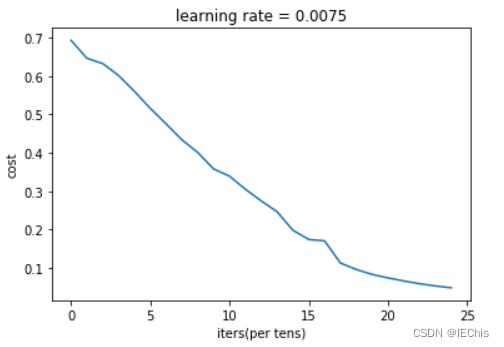
params = two_layer_model(train_x,train_y,layers_dims = (n_x,n_h,n_y),num_iters=2500,print_cost=True,isPlot=True)

所得结果如下

0 次的成本为： 0.6930497356599891
100 次的成本为： 0.6464320953428849
200 次的成本为： 0.6325140647912677
300 次的成本为： 0.6015024920354665
400 次的成本为： 0.5601966311605748
500 次的成本为： 0.515830477276473
600 次的成本为： 0.47549013139433266
700 次的成本为： 0.43391631512257495
800 次的成本为： 0.400797753620389
900 次的成本为： 0.3580705011323798
1000 次的成本为： 0.3394281538366412
1100 次的成本为： 0.3052753636196264
1200 次的成本为： 0.2749137728213017
1300 次的成本为： 0.2468176821061485
1400 次的成本为： 0.19850735037466108
1500 次的成本为： 0.174483181125566
1600 次的成本为： 0.17080762978096897
1700 次的成本为： 0.11306524562164709
1800 次的成本为： 0.09629426845937147
1900 次的成本为： 0.08342617959726864
2000 次的成本为： 0.07439078704319083
2100 次的成本为： 0.06630748132267932
2200 次的成本为： 0.05919329501038171
2300 次的成本为： 0.05336140348560558
2400 次的成本为： 0.0485547856287702

在这里插入图片描述

predict

def predict(X,y,params):
    m = X.shape[1]
    n = len(params)//2    #NN层数
    p = np.zeros((1,m))
    
    probas, caches = L_model_forward(X,params)
    
    for i in range(0,probas.shape[1]):
        if probas[0,i]>0.5:
            p[0,i] = 1
        else:
            p[0,i] = 0
    
    print("accuracy is " + str(float(np.sum((p == y)/m))))
           
    return p

使用predict验证训练集和测试集的准确度

predictions_train = predict(train_x, train_y, params) #训练集
predictions_test = predict(test_x, test_y, params) #测试集

所得结果如下

accuracy is 0.9999999999999998
accuracy is 0.72

接下来试搭建层数更多的模型，来比较准确度

L-layer NN model

# 接下来试搭建多层NN
def L_layer_model(X,Y,layer_dims,alpha=0.0075,num_iters=3000,print_cost=False,isPlot=True):
    np.random.seed(1)
    costs=[]
    
    params = ini_params_deep(layer_dims)
    
    for i in range(0,num_iters):
        AL,caches = L_model_forward(X,params)
        
        cost = compute_cost(AL,Y)
        
        grads = L_model_backward(AL,Y,caches)
        
        params = update_params(params,grads,alpha)
        
        if i % 100 ==0:
            costs.append(cost)
            if print_cost:
                print("cost of iteration " , i, " is ", np.squeeze(cost))
                
    if isPlot:
        plt.plot(np.squeeze(costs))
        plt.ylabel("cost")
        plt.xlabel("iterations (per tens)")
        plt.title("Learning rate = " + str(alpha))
        plt.show
        
    return params

用同样的数据进行训练及测试

train_set_x_orig , train_set_y , test_set_x_orig , test_set_y , classes = lr_utils.load_dataset()

train_x_flatten = train_set_x_orig.reshape(train_set_x_orig.shape[0], -1).T 
test_x_flatten = test_set_x_orig.reshape(test_set_x_orig.shape[0], -1).T

train_x = train_x_flatten / 255
train_y = train_set_y
test_x = test_x_flatten / 255
test_y = test_set_y

# 测试，做一个5层NN，每层的nueron=12288，20，7，5，1
layer_dims = [12288,20,7,5,1]
params = L_layer_model(train_x,train_y,layer_dims,num_iters=2500,print_cost=True,isPlot=True)

所得结果如下

cost of iteration  0  is  0.715731513413713
cost of iteration  100  is  0.6747377593469114
cost of iteration  200  is  0.6603365433622128
cost of iteration  300  is  0.6462887802148751
cost of iteration  400  is  0.6298131216927773
cost of iteration  500  is  0.6060056229265339
cost of iteration  600  is  0.5690041263975134
cost of iteration  700  is  0.519796535043806
cost of iteration  800  is  0.46415716786282285
cost of iteration  900  is  0.40842030048298916
cost of iteration  1000  is  0.37315499216069037
cost of iteration  1100  is  0.3057237457304712
cost of iteration  1200  is  0.2681015284774084
cost of iteration  1300  is  0.23872474827672593
cost of iteration  1400  is  0.20632263257914712
cost of iteration  1500  is  0.17943886927493546
cost of iteration  1600  is  0.15798735818801213
cost of iteration  1700  is  0.1424041301227393
cost of iteration  1800  is  0.12865165997885838
cost of iteration  1900  is  0.11244314998155497
cost of iteration  2000  is  0.08505631034966696
cost of iteration  2100  is  0.05758391198605791
cost of iteration  2200  is  0.0445675345469387
cost of iteration  2300  is  0.03808275166597669
cost of iteration  2400  is  0.034410749018403054

$[外链图片转存失败,源站可能有防盗链机制,建议将图片保存下来直接上传(img-kbIxIaWV-1662180469904)(C:\Users\JUMP_C\AppData\Roaming\Typora\typora-user-images\image-20220903124035996.png)]$

用predict验证训练集和测试集的准确度

pred_train = predict(train_x, train_y, params) #训练集
pred_test = predict(test_x, test_y, params) #测试集

所得结果如下

accuracy is 0.9952153110047844
accuracy is 0.78

通过比较，发现多层模型在测试集的表现更好。（0.72->0.78）

3.应用测试与错误分析

applicate

可以导入自己的猫猫图片进行测试

# 测试自己的图
fname = "D:\DL\C1WEEK4\my_image.png"
image = plt.imread(fname)
plt.imshow(image)
my_label_y = [1]
image.shape

#输出结果
(336, 333, 3)

$[外链图片转存失败,源站可能有防盗链机制,建议将图片保存下来直接上传(img-lZbV5lfz-1662180469905)(D:\DL\C1WEEK4\my_image.png)]$

查看图片格式发现与我们的模型并不相符，所以需要进行格式转化

from skimage import transform
image_trans = transform.resize(image,(64,64,3)).reshape(64*64*3,1)
image_trans.shape

#输出结果
(12288, 1)

然后就可以进行预测了

my_prediction = predict(image_trans,my_label_y,params)
print("y = " + str(np.squeeze(my_prediction)))

#输出结果
accuracy is 1.0
y = 1.0

error analysis

# 可以进一步分析错误样本，寻找影响准确率的因素
def print_mislabeled_images(classes,X,y,p):
    a = p + y
    mislabeled_indices = np.asarray(np.where(a == 1))
    plt.rcParams["figure.figsize"] = (40.0,40.0)
    num_images = len(mislabeled_indices[0])
    for i in range(num_images):
        index = mislabeled_indices[1][i]
        
        plt.subplot(2,num_images,i+1)
        plt.imshow(X[:,index].reshape(64,64,3),interpolation='nearest')
        plt.axis('off')
        plt.title("Predictioin: " + classes[int(p[0,index])].decode("utf-8") + "\n Class: "+ classes[y[0,index]].decode("utf-8"))
        
print_mislabeled_images(classes,test_x,test_y,pred_test)

输出结果

$[外链图片转存失败,源站可能有防盗链机制,建议将图片保存下来直接上传(img-DHX37XwO-1662180469905)(C:\Users\JUMP_C\AppData\Roaming\Typora\typora-user-images\image-20220903123452005.png)]$

IEChis

关注

0
点赞
踩
0

收藏

觉得还不错? 一键收藏
0
评论
Deep learning practice of ANg(C1week4))

目的：搭建多层神经网络分析：如上次作业，并构建好、、、的基本函数。注意初始化参数时w的初始化与上次的不同。先将功能拆分实现，再进行组合，就可以完成一个。最后可以试试，以及进行。
复制链接

扫一扫