R2周-LSTM-火灾温度预测

•  🍨 本文为🔗365天深度学习训练营 中的学习记录博客
• 🍖 作者：K同学啊
• 电脑系统：Windows 10
• 语言环境：Python 3.8.5
• 编译器：Pycharm 2022.02
• 深度学习环境：TensorFlow 2.10.0
• 显卡及显存：RTX 3060 12G

目录

目录

前言

一、数据集

二、前期工作

1、默认启动GPU，没有的话则使用CPU

2、读入数据

3、数据可视化

三、数据预处理

1.设置X,y

2、划分数据集

3、数据归一化

四、构建LSTM网络

1、函数模型

2、构建函数模型

五、训练模型

1、超参数

2、训练函数

3、模型评估

4、测试集预测

5、均方根误差和R2

总结

参考资料

---

前言

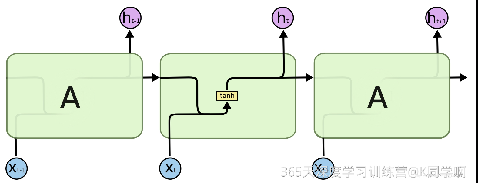
 RNN原理:在标准 RNN 中，这个重复模块将具有非常简单的结构，例如单个 tanh 层

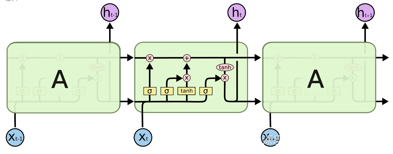
 LSTM原理:通过门控状态来选择调整传输的信息，简单的来说就是记住需要长时间记忆的信息，忘记不重要的信息，其结构如下：

一、数据集

​

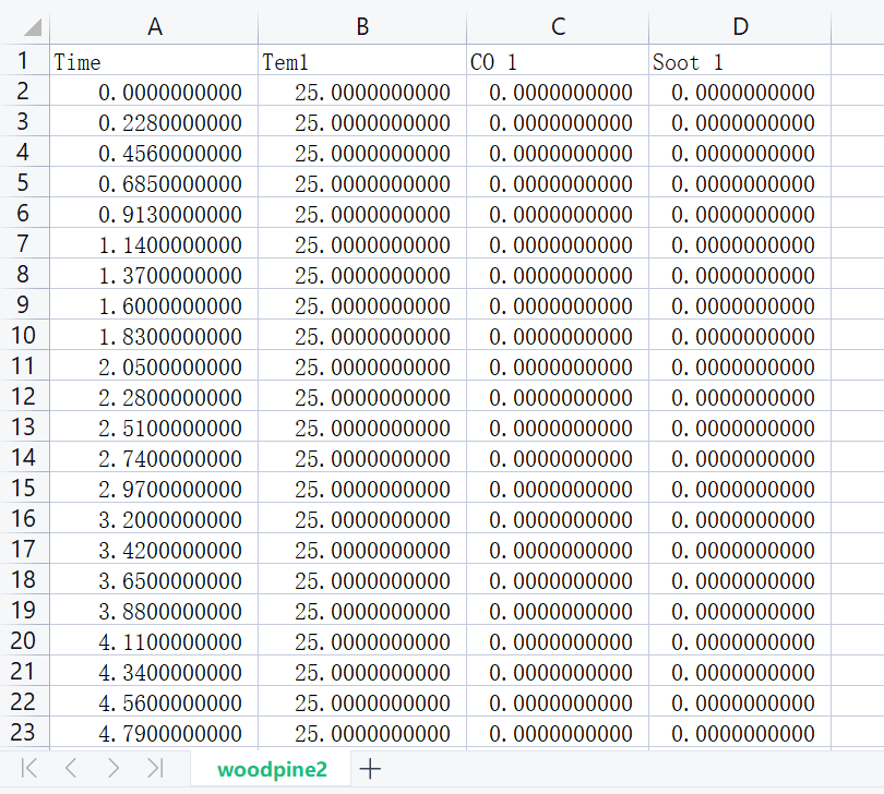
其中每个数据的标签含义为：

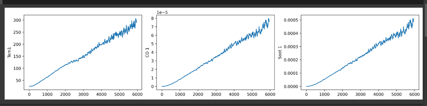
• Time：时间
• Tem1：火灾温度
• CO 1：一氧化碳浓度
• Soot 1：烟雾浓度

二、前期工作

1、默认启动GPU，没有的话则使用CPU

代码如下（示例）：

import tensorflow as tf

gpus = tf.config.list_physical_devices("GPU")

if gpus:
    gpu0 = gpus[0]                                        #如果有多个GPU，仅使用第0个GPU
    tf.config.experimental.set_memory_growth(gpu0, True)  #设置GPU显存用量按需使用
    tf.config.set_visible_devices([gpu0],"GPU")

2、读入数据

import pandas as pd
import numpy as np

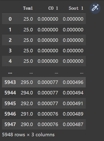
df = pd.read_csv("E:\DL_data\Day21\heart.csv")
dataFrame = df.iloc[:,1:]
dataFrame

 

3、数据可视化

import matplotlib.pyplot as plt
import seaborn as sns

plt.rcParams['savefig.dpi'] = 500 #图片像素
plt.rcParams['figure.dpi']  = 500 #分辨率

fig, ax =plt.subplots(1,3,constrained_layout=True, figsize=(14, 3))

sns.lineplot(data=df["Tem1"], ax=ax[0])
sns.lineplot(data=df["CO 1"], ax=ax[1])
sns.lineplot(data=df["Soot 1"], ax=ax[2])
plt.show()

三、数据预处理

1.设置X,y

width_X = 8
width_y = 1

X = []
y = []

in_start = 0

for _, _ in df.iterrows():
    in_end  = in_start + width_X
    out_end = in_end   + width_y

    if out_end < len(dataFrame):
        X_ = np.array(dataFrame.iloc[in_start:in_end , ])
        X_ = X_.reshape((len(X_)*3))
        y_ = np.array(dataFrame.iloc[in_end  :out_end, 0])

        X.append(X_)
        y.append(y_)

    in_start += 1

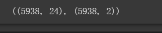
X = np.array(X)
y = np.array(y)

X.shape, y.shape

2、划分数据集

from sklearn.preprocessing import StandardScaler
from sklearn.model_selection import train_test_split

x = df.iloc[:,:-1]
y = df.iloc[:,-1]

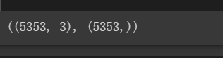
x_train, x_test, y_train, y_test = train_test_split(x, y, test_size=0.1, random_state=1)

x_train.shape, y_train.shape

2、数据归一化

from sklearn.preprocessing import MinMaxScaler

#将数据归一化，范围是0到1
sc       = MinMaxScaler(feature_range=(0, 1))
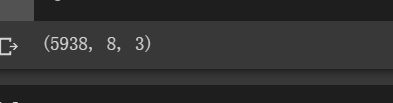
X_scaled = sc.fit_transform(X)
X_scaled = X_scaled.reshape(len(X_scaled),width_X,3)
X_scaled.shape

四、构建LSTM网络

1、函数模型

tf.keras.layers.LSTM(
    units,
    activation='tanh',
    recurrent_activation='sigmoid',
    use_bias=True,
    kernel_initializer='glorot_uniform',
    recurrent_initializer='orthogonal',
    bias_initializer='zeros',
    unit_forget_bias=True,
    kernel_regularizer=None,
    recurrent_regularizer=None,
    bias_regularizer=None,
    activity_regularizer=None,
    kernel_constraint=None,
    recurrent_constraint=None,
    bias_constraint=None,
    dropout=0.0,
    recurrent_dropout=0.0,
    return_sequences=False,
    return_state=False,
    go_backwards=False,
    stateful=False,
    time_major=False,
    unroll=False,
    **kwargs
)

​

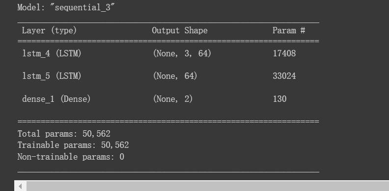
2、构建函数模型

from tensorflow.keras.models import Sequential
from tensorflow.keras.layers import Dense,LSTM

# 多层 LSTM
model_lstm = Sequential()
model_lstm.add(LSTM(units=64, activation='relu', return_sequences=True,
                    input_shape=(X_train.shape[1], 3)))
model_lstm.add(LSTM(units=64, activation='relu'))

model_lstm.add(Dense(width_y))

​

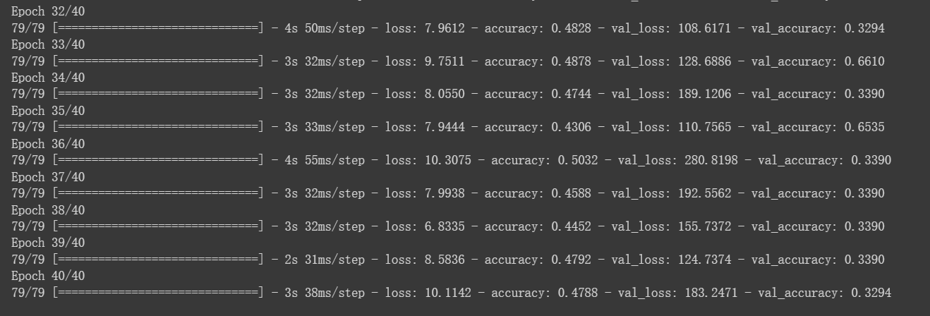
五、训练模型

1、超参数

opt = tf.keras.optimizers.Adam(learning_rate=1e-4)
model.compile(loss='binary_crossentropy', optimizer=opt,metrics=['accuracy'])

2、训练函数

history = model_lstm.fit(X_train, y_train, batch_size = 64, epochs = 40, validation_data = (X_test, y_test), validation_freq = 1)

​

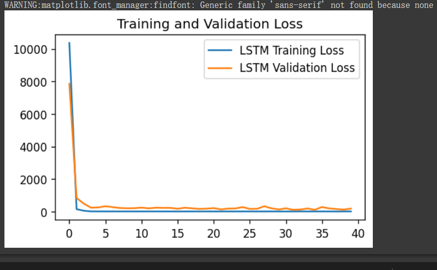
3、模型评估

import matplotlib.pyplot as plt

acc = history.history['accuracy']
val_acc = history.history['val_accuracy']

loss = history.history['loss']
val_loss = history.history['val_loss']

epochs_range = range(epochs)

plt.figure(figsize=(14, 4))
plt.subplot(1, 2, 1)

plt.plot(epochs_range, acc, label='Training Accuracy')
plt.plot(epochs_range, val_acc, label='Validation Accuracy')
plt.legend(loc='lower right')
plt.title('Training and Validation Accuracy')

plt.subplot(1, 2, 2)
plt.plot(epochs_range, loss, label='Training Loss')
plt.plot(epochs_range, val_loss, label='Validation Loss')
plt.legend(loc='upper right')
plt.title('Training and Validation Loss')
plt.show()

​

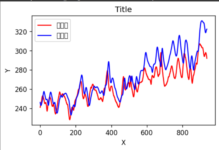
4、测试集预测

5、均方根误差和R2

from sklearn import metrics
"""
RMSE ：均方根误差,对均方误差开方
R2   ：决定系数，可以简单理解为反映模型拟合优度的重要的统计量
"""
RMSE_lstm  = metrics.mean_squared_error(predicted_y_lstm, y_test)**0.5
R2_lstm    = metrics.r2_score(predicted_y_lstm, y_test)

print('均方根误差: %.5f' % RMSE_lstm)
print('R2: %.5f' % R2_lstm)

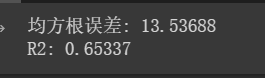
RMSE均方根误差是预测值与真实值的误差平方根的均值，它用来估计模型预测目标值的性能（准确度），值越小，模型的质量越好。

R2是将预测值跟只使用均值的情况下相比，看能好多少。其区间通常在（0,1）之间。0表示还不如什么都不预测，直接取均值的情况，而1表示所有预测跟真实结果完美匹配的情况，值越接近1，模型的质量越好

总结

文章主要包括以下几个部分：

1. 数据集介绍：介绍了所使用的火灾数据集，包括数据集的标签含义等。
2. 前期工作：包括默认启动GPU，读入数据以及对数据进行可视化的操作。
3. 数据预处理：对数据进行归一化操作，并将数据集划分为训练集和测试集。
4. 构建LSTM网络：介绍了如何使用TensorFlow中的LSTM函数来构建函数模型。
5. 训练模型：介绍了模型的超参数设置以及如何进行模型训练。

参考资料

循环神经网络RNN以及几种经典模型
深度学习 Day22——利用LSTM实现火灾温度预测