


一、梯度下降:梯度下降是一种优化算法,用于找到函数的局部最小值。它通过沿着梯度的反方向迭代更新参数,以降低目标函数的值。
代码:
from sklearn.datasets import load_iris
from sklearn.tree import DecisionTreeClassifier
from sklearn.model_selection import train_test_split, GridSearchCV
from sklearn.metrics import accuracy_score, confusion_matrix
import matplotlib.pyplot as plt
import numpy as np
# 加载鸢尾花数据集
iris = load_iris()
X = iris.data
y = iris.target
# 将数据集分割为训练集和测试集
X_train, X_test, y_train, y_test = train_test_split(X, y, test_size=0.2, random_state=42)
# 定义网格搜索的超参数范围
param_grid = {
'max_depth': [3, 5, 7, None],
'min_samples_split': [2, 5, 10],
'min_samples_leaf': [1, 2, 4],
'criterion': ['gini', 'entropy']
}
# 初始化GridSearchCV
grid_search = GridSearchCV(estimator=DecisionTreeClassifier(), param_grid=param_grid, cv=5)
# 将网格搜索适配到数据集上
grid_search.fit(X_train, y_train)
# 获取网格搜索结果
results = grid_search.cv_results_
param_names = list(param_grid.keys())
params_combinations = results['params']
mean_test_scores = results['mean_test_score']
# 打印出最佳超参数
print("最佳超参数:", grid_search.best_params_)
# 获取最佳模型
best_clf = grid_search.best_estimator_
# 评估最佳模型
y_pred = best_clf.predict(X_test)
accuracy = accuracy_score(y_test, y_pred)
print("准确率:", accuracy)
# 计算混淆矩阵
conf_matrix = confusion_matrix(y_test, y_pred)
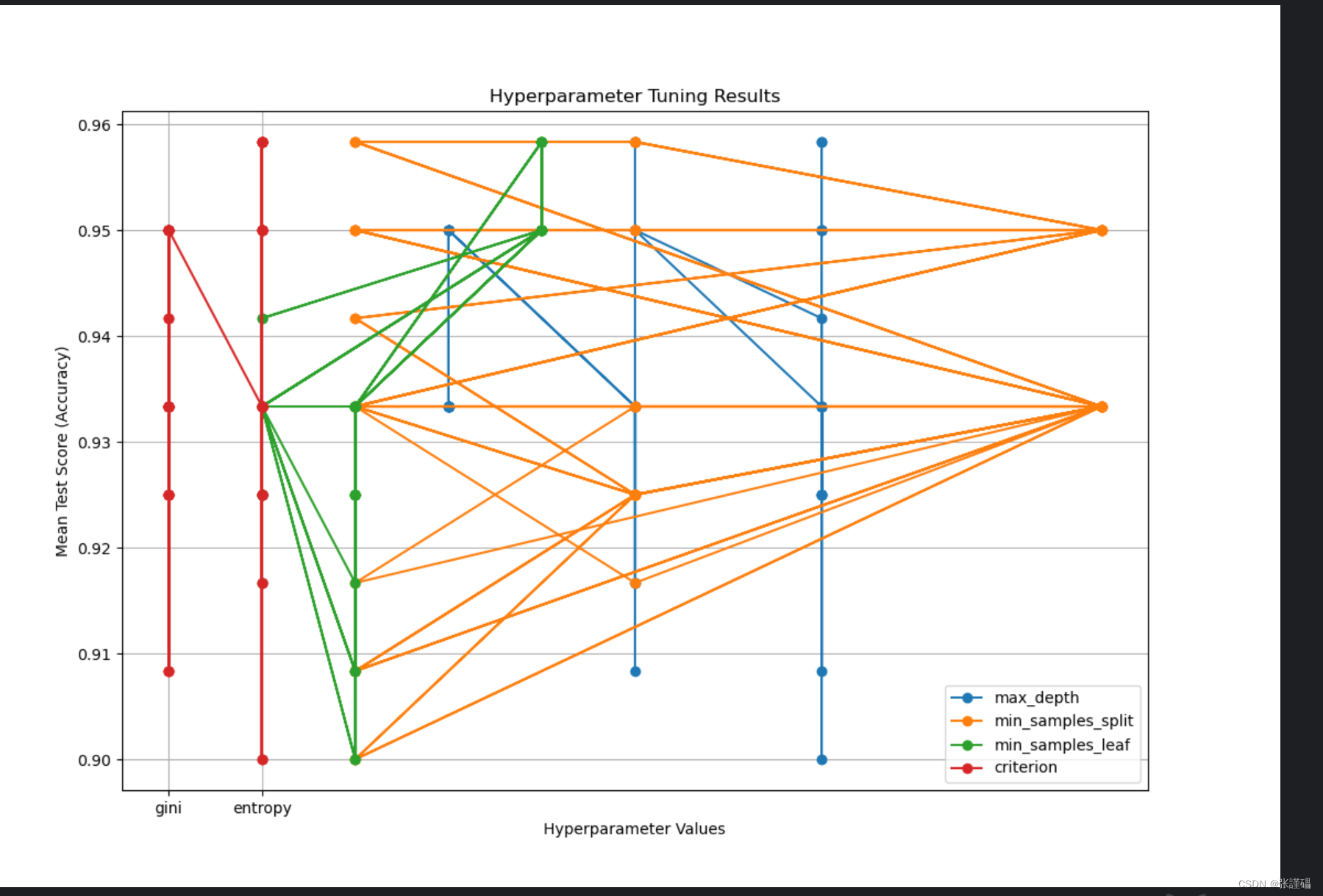
# 生成折线图
plt.figure(figsize=(12, 8))
for i, param in enumerate(param_names):
param_values = [x[param] for x in params_combinations] # 获取对应超参数的取值
plt.plot(param_values, mean_test_scores, marker='o', label=f'{param}')
plt.title('Hyperparameter Tuning Results')
plt.xlabel('Hyperparameter Values')
plt.ylabel('Mean Test Score (Accuracy)')
plt.legend()
plt.grid(True)
plt.show()
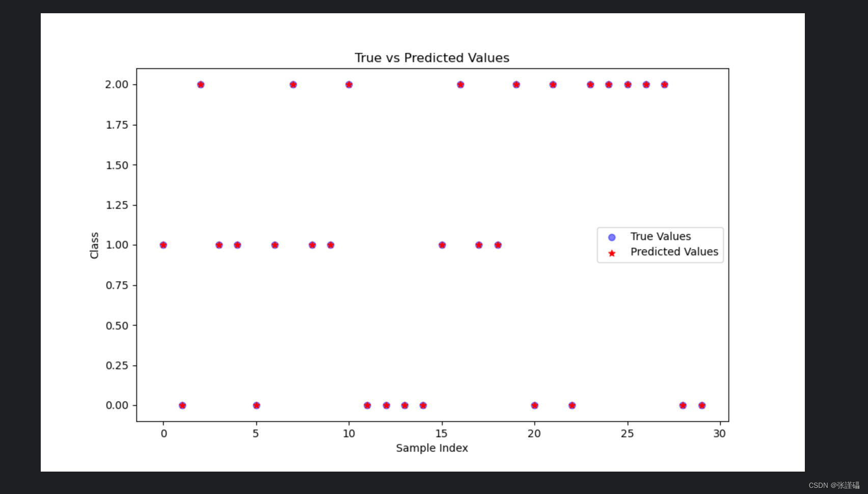
# 生成真实值和预测值对比的图表
plt.figure(figsize=(10, 6))
plt.scatter(np.arange(len(y_test)), y_test, color='blue', label='True Values', alpha=0.5)
plt.scatter(np.arange(len(y_test)), y_pred, color='red', label='Predicted Values', alpha=1,marker='*')
plt.title('True vs Predicted Values')
plt.xlabel('Sample Index')
plt.ylabel('Class')
plt.legend()
plt.show()
# 输出混淆矩阵
print("混淆矩阵:")
print(conf_matrix) 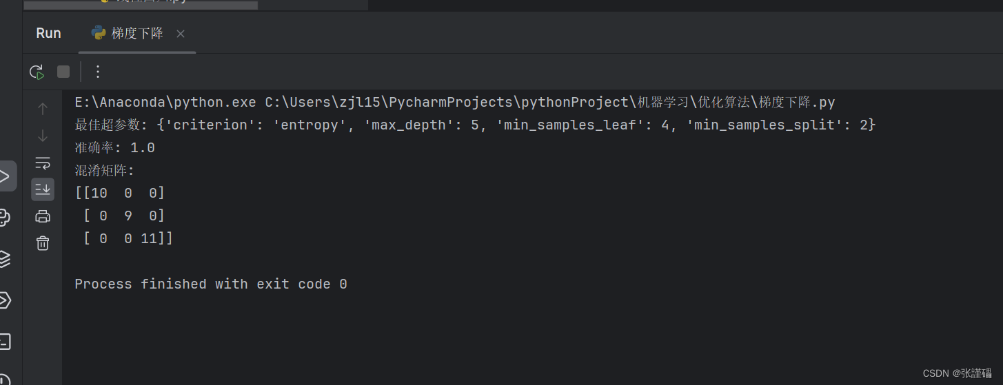
二、牛顿法:牛顿法是一种迭代优化算法,通过使用函数的二阶导数信息来更新参数,以更快地收敛到函数的极小值点。
代码:
from sklearn.datasets import load_iris
from sklearn.tree import DecisionTreeClassifier
from sklearn.model_selection import train_test_split
from sklearn.metrics import accuracy_score, confusion_matrix
import matplotlib.pyplot as plt
import numpy as np
from scipy.optimize import minimize

# 加载鸢尾花数据集
iris = load_iris()
X = iris.data
y = iris.target

# 将数据集分割为训练集和测试集
X_train, X_test, y_train, y_test = train_test_split(X, y, test_size=0.2, random_state=42)


# 定义交叉熵损失函数和其梯度
def cross_entropy_loss(theta, X, y):
    # 提取决策树的参数
    max_depth, min_samples_split, min_samples_leaf = theta

    # 将min_samples_leaf转换为整数
    min_samples_leaf = int(min_samples_leaf)

    # 训练决策树
    clf = DecisionTreeClassifier(max_depth=max_depth, min_samples_split=min_samples_split,
                                 min_samples_leaf=min_samples_leaf)
    clf.fit(X, y)

    # 计算交叉熵损失
    y_pred_proba = clf.predict_proba(X)
    loss = -np.sum(np.log(y_pred_proba[np.arange(len(y)), y])) / len(y)

    return loss


def cross_entropy_gradient(theta, X, y):
    # 提取决策树的参数
    max_depth, min_samples_split, min_samples_leaf = theta

    # 将min_samples_leaf转换为整数
    min_samples_leaf = int(min_samples_leaf)

    # 训练决策树
    clf = DecisionTreeClassifier(max_depth=max_depth, min_samples_split=min_samples_split,
                                 min_samples_leaf=min_samples_leaf)
    clf.fit(X, y)

    # 计算预测概率
    y_pred_proba = clf.predict_proba(X)

    # 计算交叉熵损失的梯度
    grad = np.zeros(3)
    for i in range(len(X)):
        for k in range(3):
            if k == y[i]:
                grad[0] += -(1 - y_pred_proba[i, k]) * X[i, 0]
                grad[1] += -(1 - y_pred_proba[i, k]) * X[i, 1]
                grad[2] += -(1 - y_pred_proba[i, k]) * X[i, 2]
            else:
                grad[0] += y_pred_proba[i, k] * X[i, 0]
                grad[1] += y_pred_proba[i, k] * X[i, 1]
                grad[2] += y_pred_proba[i, k] * X[i, 2]

    grad /= len(y)

    return grad


# 初始化参数
theta_initial = [3, 2, 1]

# 使用牛顿法最小化交叉熵损失函数
result = minimize(cross_entropy_loss, theta_initial, args=(X_train, y_train), jac=cross_entropy_gradient,
                  method='Newton-CG')

# 获取最优参数
max_depth_opt, min_samples_split_opt, min_samples_leaf_opt = result.x

# 将最优min_samples_leaf转换为整数
min_samples_leaf_opt = int(min_samples_leaf_opt)

# 构建最优模型
best_clf = DecisionTreeClassifier(max_depth=max_depth_opt, min_samples_split=min_samples_split_opt,
                                  min_samples_leaf=min_samples_leaf_opt)
best_clf.fit(X_train, y_train)

# 评估最佳模型
y_pred = best_clf.predict(X_test)
accuracy = accuracy_score(y_test, y_pred)
print("准确率:", accuracy)

# 计算混淆矩阵
conf_matrix = confusion_matrix(y_test, y_pred)

# 输出混淆矩阵
print("混淆矩阵:")
print(conf_matrix)
三、拟牛顿法:拟牛顿法是一类使用函数的一阶导数信息和历史迭代信息来近似二阶导数的优化算法。它通过更新拟牛顿矩阵来逼近牛顿法的迭代过程,从而减少计算二阶导数的开销。
代码:
import numpy as np
from scipy.optimize import minimize
from sklearn.datasets import load_iris
from sklearn.model_selection import train_test_split
from sklearn.tree import DecisionTreeClassifier

# Load the Iris dataset
iris = load_iris()
X = iris.data
y = iris.target

# Split the dataset into training and testing sets
X_train, X_test, y_train, y_test = train_test_split(X, y, test_size=0.2, random_state=42)

# Define cross-entropy loss function
def cross_entropy_loss(theta, X, y):
    clf = DecisionTreeClassifier(min_samples_split=int(theta[0]))
    clf.fit(X, y)
    y_pred = clf.predict_proba(X)
    loss = -np.mean(np.log(y_pred[np.arange(len(y)), y]))
    return loss

# Define gradient of cross-entropy loss function
def cross_entropy_gradient(theta, X, y):
    clf = DecisionTreeClassifier(min_samples_split=int(theta[0]))
    clf.fit(X, y)
    y_pred = clf.predict_proba(X)
    grad = np.zeros_like(theta)
    for i in range(len(grad)):
        clf.min_samples_split = int(theta[0] + 1e-6)
        y_pred_plus = clf.predict_proba(X)
        clf.min_samples_split = int(theta[0] - 1e-6)
        y_pred_minus = clf.predict_proba(X)
        grad[i] = -np.mean((y_pred_plus - y_pred_minus) * (y == i)[:, np.newaxis])
    return grad

# Initial guess for theta
theta_initial = np.array([2.0])  # Initial value for min_samples_split

# Perform optimization using BFGS
result = minimize(cross_entropy_loss, theta_initial, args=(X_train, y_train), jac=cross_entropy_gradient,
                  method='BFGS')

# Get the optimal value of theta
optimal_theta = result.x

# Train the classifier with the optimal min_samples_split value
optimal_clf = DecisionTreeClassifier(min_samples_split=int(optimal_theta))
optimal_clf.fit(X_train, y_train)

# Evaluate the classifier on the testing data
accuracy = optimal_clf.score(X_test, y_test)
print("Optimal min_samples_split:", int(optimal_theta))
print("Accuracy:", accuracy)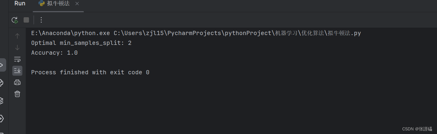
四、共轭梯度法:共轭梯度法是一种用于解决大规模线性方程组或最小化二次型函数的优化算法。它利用了不同方向上的梯度共轭性质,在每一步迭代中找到一个共轭方向,并沿着该方向进行参数更新,以加快收敛速度。
代码:
from sklearn.datasets import load_iris
from sklearn.linear_model import LogisticRegression
from sklearn.model_selection import train_test_split, GridSearchCV
from sklearn.metrics import accuracy_score, confusion_matrix
import matplotlib.pyplot as plt
import numpy as np
# 加载鸢尾花数据集
iris = load_iris()
X = iris.data
y = iris.target
# 将数据集分割为训练集和测试集
X_train, X_test, y_train, y_test = train_test_split(X, y, test_size=0.2, random_state=42)
# 定义网格搜索的超参数范围
param_grid = {
'C': [0.001, 0.01, 0.1, 1, 10, 100], # 正则化参数
'penalty': ['l2'], # 正则化类型,这里选择L2正则化
'solver': ['lbfgs'], # 选择共轭梯度法优化器
}
# 初始化GridSearchCV
grid_search = GridSearchCV(estimator=LogisticRegression(), param_grid=param_grid, cv=5)
# 将网格搜索适配到数据集上
grid_search.fit(X_train, y_train)
# 获取网格搜索结果
results = grid_search.cv_results_
param_names = list(param_grid.keys())
params_combinations = results['params']
mean_test_scores = results['mean_test_score']
# 打印出最佳超参数
print("最佳超参数:", grid_search.best_params_)
# 获取最佳模型
best_clf = grid_search.best_estimator_
# 评估最佳模型
y_pred = best_clf.predict(X_test)
accuracy = accuracy_score(y_test, y_pred)
print("准确率:", accuracy)
# 计算混淆矩阵
conf_matrix = confusion_matrix(y_test, y_pred)
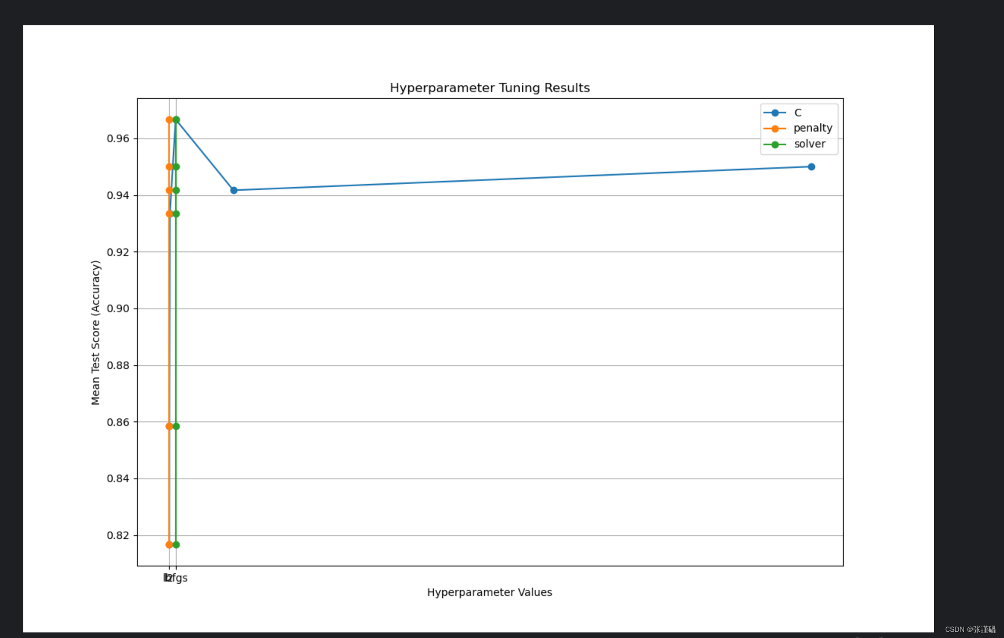
# 生成折线图
plt.figure(figsize=(12, 8))
for i, param in enumerate(param_names):
param_values = [x[param] for x in params_combinations] # 获取对应超参数的取值
plt.plot(param_values, mean_test_scores, marker='o', label=f'{param}')
plt.title('Hyperparameter Tuning Results')
plt.xlabel('Hyperparameter Values')
plt.ylabel('Mean Test Score (Accuracy)')
plt.legend()
plt.grid(True)
plt.show()
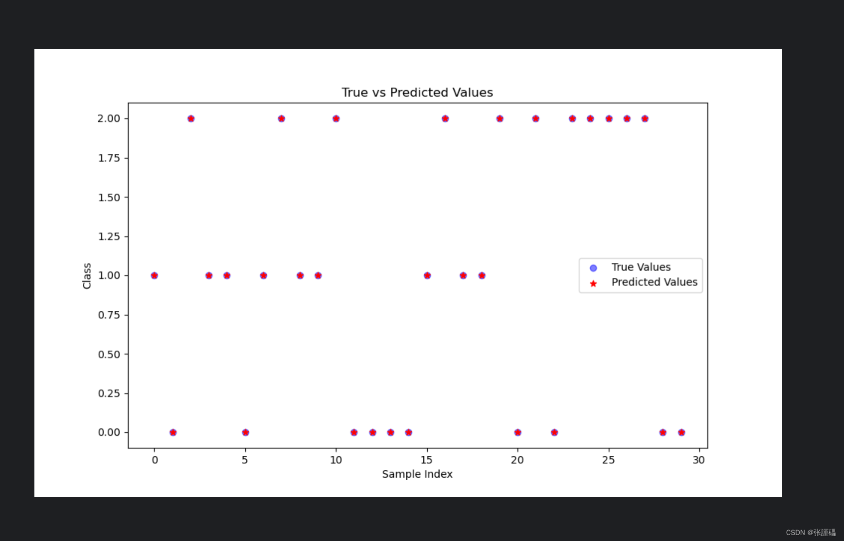
# 生成真实值和预测值对比的图表
plt.figure(figsize=(10, 6))
plt.scatter(np.arange(len(y_test)), y_test, color='blue', label='True Values', alpha=0.5)
plt.scatter(np.arange(len(y_test)), y_pred, color='red', label='Predicted Values', alpha=1,marker='*')
plt.title('True vs Predicted Values')
plt.xlabel('Sample Index')
plt.ylabel('Class')
plt.legend()
plt.show()
# 输出混淆矩阵
print("混淆矩阵:")
print(conf_matrix)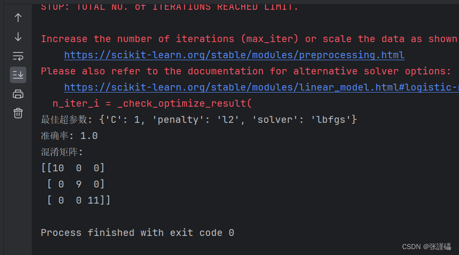


 4万+
4万+


 被折叠的 条评论
为什么被折叠?
被折叠的 条评论
为什么被折叠?
 到【灌水乐园】发言


