Machine Learning Mastery 计算机视觉教程（三）

原文：Machine Learning Mastery

协议：CC BY-NC-SA 4.0

如何为 MNIST 手写数字分类开发 CNN

原文：https://machinelearningmastery.com/how-to-develop-a-convolutional-neural-network-from-scratch-for-mnist-handwritten-digit-classification/

最后更新于 2021 年 11 月 14 日

如何从头开发卷积神经网络用于 MNIST 手写数字分类？

MNIST 手写数字分类问题是用于计算机视觉和深度学习的标准数据集。

虽然数据集得到了有效解决，但它可以作为学习和实践如何从零开始开发、评估和使用卷积深度学习神经网络进行图像分类的基础。这包括如何开发一个健壮的测试工具来评估模型的表现，如何探索模型的改进，以及如何保存模型并在以后加载它来对新数据进行预测。

在本教程中，您将发现如何从零开始开发用于手写数字分类的卷积神经网络。

完成本教程后，您将知道:

• 如何开发一个测试工具来开发一个健壮的模型评估，并为分类任务建立一个表现基线。
• 如何探索基线模型的扩展，以提高学习和模型能力。
• 如何开发最终模型，评估最终模型的表现，并使用它对新图像进行预测。

用我的新书计算机视觉深度学习启动你的项目，包括分步教程和所有示例的 Python 源代码文件。

我们开始吧。

• 2019 年 12 月更新:更新了 TensorFlow 2.0 和 Keras 2.3 的示例。
• 2020 年 1 月更新:修复了在交叉验证循环之外定义模型的 bug。
• 2021 年 11 月更新:更新使用 Tensorflow 2.6

如何从零开始开发卷积神经网络用于 MNIST 手写数字分类
图片由理查德·阿拉维提供，版权所有。

教程概述

本教程分为五个部分；它们是:

1. MNIST 手写数字类别数据集
2. 模型评估方法
3. 如何开发基线模型
4. 如何开发改进的模型
5. 如何最终确定模型并做出预测

发展环境

本教程假设您正在使用独立的 Keras，它运行在 Python 3 的 TensorFlow 之上。如果您需要设置开发环境的帮助，请参阅本教程:

• 如何用 Anaconda 设置机器学习的 Python 环境

MNIST 手写数字类别数据集

MNIST 数据集是一个首字母缩略词，代表修改后的国家标准和技术研究所数据集。

它是一个由 60，000 个 0 到 9 之间的手写单个数字的 28×28 像素小正方形灰度图像组成的数据集。

任务是将手写数字的给定图像分类为代表从 0 到 9 的整数值的 10 个类别之一。

这是一个被广泛使用和深入理解的数据集，并且在很大程度上是“解决了”表现最好的模型是深度学习卷积神经网络，其分类准确率达到 99%以上，在等待测试数据集上的错误率在 0.4%到 0.2%之间。

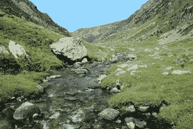
以下示例使用 Keras API 加载 MNIST 数据集，并创建训练数据集中前九幅图像的图。

# example of loading the mnist dataset
from tensorflow.keras.datasets import mnist
from matplotlib import pyplot as plt
# load dataset
(trainX, trainy), (testX, testy) = mnist.load_data()
# summarize loaded dataset
print('Train: X=%s, y=%s' % (trainX.shape, trainy.shape))
print('Test: X=%s, y=%s' % (testX.shape, testy.shape))
# plot first few images
for i in range(9):
	# define subplot
	plt.subplot(330 + 1 + i)
	# plot raw pixel data
	plt.imshow(trainX[i], cmap=plt.get_cmap('gray'))
# show the figure
plt.show()

运行该示例将加载 MNIST 训练和测试数据集，并打印它们的形状。

我们可以看到训练数据集中有 6 万个例子，测试数据集中有 1 万个例子，图像确实是 28×28 像素的正方形。

Train: X=(60000, 28, 28), y=(60000,)
Test: X=(10000, 28, 28), y=(10000,)

还创建了数据集中前九幅图像的图，显示了要分类的图像的自然手写特性。

从 MNIST 数据集绘制图像子集

模型评估方法

尽管有效地解决了 MNIST 数据集，但是它可以成为开发和实践使用卷积神经网络解决图像分类任务的方法的有用的起点。

我们可以从零开始开发一个新的模型，而不是回顾数据集上表现良好的模型的文献。

数据集已经有了我们可以使用的定义良好的训练和测试数据集。

为了估计给定训练运行的模型表现，我们可以进一步将训练集拆分为训练和验证数据集。然后，可以绘制每次运行的训练和验证数据集的表现，以提供学习曲线和对模型学习问题的深入了解。

Keras API 通过在训练模型时为 model.fit() 函数指定“ validation_data ”参数来支持这一点，该函数将返回一个对象，该对象描述所选损失的模型表现和每个训练时期的度量。

# record model performance on a validation dataset during training
history = model.fit(..., validation_data=(valX, valY))

为了估计一个模型在一般问题上的表现，我们可以使用 k 倍交叉验证，也许是五倍交叉验证。这将给出关于训练和测试数据集的差异以及学习算法的随机性质的模型方差的一些说明。在给定标准差的情况下，模型的表现可以作为 k 倍的平均表现，如果需要，可以用来估计置信区间。

我们可以使用 Sklearn API 中的 KFold 类来实现给定神经网络模型的 K 折交叉验证评估。有许多方法可以实现这一点，尽管我们可以选择一种灵活的方法，其中 KFold 类仅用于指定用于每个 spit 的行索引。

# example of k-fold cv for a neural net
data = ...
# prepare cross validation
kfold = KFold(5, shuffle=True, random_state=1)
# enumerate splits
for train_ix, test_ix in kfold.split(data):
        model = ...
	...

我们将保留实际的测试数据集，并将其用作最终模型的评估。

如何开发基线模型

第一步是开发一个基线模型。

这一点至关重要，因为它既涉及到为测试工具开发基础设施，以便我们设计的任何模型都可以在数据集上进行评估，又建立了问题模型表现的基线，通过该基线可以比较所有的改进。

测试线束的设计是模块化的，我们可以为每个部件开发单独的功能。如果我们愿意的话，这允许测试装具的给定方面独立于其他方面进行修改或交互改变。

我们可以用五个关键元素来开发这个测试工具。它们是数据集的加载、数据集的准备、模型的定义、模型的评估和结果的呈现。

加载数据集

我们知道一些关于数据集的事情。

例如，我们知道图像都是预对齐的(例如，每个图像只包含一个手绘数字)，图像都具有相同的 28×28 像素的正方形大小，并且图像是灰度级的。

因此，我们可以加载图像并重塑数据阵列，使其具有单一颜色通道。

# load dataset
(trainX, trainY), (testX, testY) = mnist.load_data()
# reshape dataset to have a single channel
trainX = trainX.reshape((trainX.shape[0], 28, 28, 1))
testX = testX.reshape((testX.shape[0], 28, 28, 1))

我们还知道有 10 个类，类被表示为唯一的整数。

因此，我们可以对每个样本的类元素使用一个热编码，将整数转换为一个 10 元素的二进制向量，类值的索引为 1，所有其他类的索引为 0。我们可以通过*到 _ classic()*效用函数来实现。

# one hot encode target values
trainY = to_categorical(trainY)
testY = to_categorical(testY)

load_dataset() 函数实现了这些行为，可以用来加载数据集。

# load train and test dataset
def load_dataset():
	# load dataset
	(trainX, trainY), (testX, testY) = mnist.load_data()
	# reshape dataset to have a single channel
	trainX = trainX.reshape((trainX.shape[0], 28, 28, 1))
	testX = testX.reshape((testX.shape[0], 28, 28, 1))
	# one hot encode target values
	trainY = to_categorical(trainY)
	testY = to_categorical(testY)
	return trainX, trainY, testX, testY

准备像素数据

我们知道，数据集中每个图像的像素值都是介于黑白或 0 到 255 之间的无符号整数。

我们不知道缩放用于建模的像素值的最佳方式，但是我们知道需要一些缩放。

一个好的起点是归一化灰度图像的像素值，例如将它们重新缩放到范围[0，1]。这包括首先将数据类型从无符号整数转换为浮点数，然后将像素值除以最大值。

# convert from integers to floats
train_norm = train.astype('float32')
test_norm = test.astype('float32')
# normalize to range 0-1
train_norm = train_norm / 255.0
test_norm = test_norm / 255.0

下面的 prep_pixels() 函数实现了这些行为，并提供了需要缩放的训练和测试数据集的像素值。

# scale pixels
def prep_pixels(train, test):
	# convert from integers to floats
	train_norm = train.astype('float32')
	test_norm = test.astype('float32')
	# normalize to range 0-1
	train_norm = train_norm / 255.0
	test_norm = test_norm / 255.0
	# return normalized images
	return train_norm, test_norm

在任何建模之前，必须调用该函数来准备像素值。

定义模型

接下来，我们需要为这个问题定义一个基线卷积神经网络模型。

该模型有两个主要方面:由卷积层和池化层组成的特征提取前端，以及进行预测的分类器后端。

对于卷积前端，我们可以从单个卷积层开始，该卷积层具有小的滤波器大小(3，3)和适度数量的滤波器(32)，然后是最大池层。过滤图然后可以被展平以向分类器提供特征。

假设问题是一个多类分类任务，我们知道我们将需要一个具有 10 个节点的输出层，以便预测属于 10 个类中每一个的图像的概率分布。这也需要使用 softmax 激活功能。在特征提取器和输出层之间，我们可以添加一个密集层来解释特征，在本例中有 100 个节点。

所有层将使用 ReLU 激活功能和 he 权重初始化方案，两者都是最佳实践。

我们将对随机梯度下降优化器使用保守配置，其学习率为 0.01，动量为 0.9。分类交叉熵损失函数将被优化，适用于多类分类，我们将监控分类准确率度量，这是适当的，因为我们在 10 类中的每一类都有相同数量的例子。

下面的 define_model() 函数将定义并返回这个模型。

# define cnn model
def define_model():
	model = Sequential()
	model.add(Conv2D(32, (3, 3), activation='relu', kernel_initializer='he_uniform', input_shape=(28, 28, 1)))
	model.add(MaxPooling2D((2, 2)))
	model.add(Flatten())
	model.add(Dense(100, activation='relu', kernel_initializer='he_uniform'))
	model.add(Dense(10, activation='softmax'))
	# compile model
	opt = SGD(learning_rate=0.01, momentum=0.9)
	model.compile(optimizer=opt, loss='categorical_crossentropy', metrics=['accuracy'])
	return model

评估模型

模型定义后，我们需要对其进行评估。

模型将使用五重交叉验证进行评估。选择 k=5 的值是为了提供重复评估的基线，并且不会大到需要很长的运行时间。每个测试集将占训练数据集的 20%，或者大约 12，000 个例子，接近于这个问题的实际测试集的大小。

训练数据集在被分割之前被混洗，并且每次都执行样本混洗，因此我们评估的任何模型将在每个文件夹中具有相同的训练和测试数据集，从而在模型之间提供苹果对苹果的比较。

我们将为一个适度的 10 个训练时期训练基线模型，默认批量为 32 个例子。每个折叠的测试集将用于在训练运行的每个时期评估模型，以便我们以后可以创建学习曲线，并在运行结束时评估模型的表现。因此，我们将跟踪每次运行的结果历史，以及折叠的分类准确率。

下面的 evaluate_model() 函数实现了这些行为，将训练数据集作为参数，并返回一个准确性分数和训练历史的列表，稍后可以对其进行总结。

# evaluate a model using k-fold cross-validation
def evaluate_model(dataX, dataY, n_folds=5):
	scores, histories = list(), list()
	# prepare cross validation
	kfold = KFold(n_folds, shuffle=True, random_state=1)
	# enumerate splits
	for train_ix, test_ix in kfold.split(dataX):
		# define model
		model = define_model()
		# select rows for train and test
		trainX, trainY, testX, testY = dataX[train_ix], dataY[train_ix], dataX[test_ix], dataY[test_ix]
		# fit model
		history = model.fit(trainX, trainY, epochs=10, batch_size=32, validation_data=(testX, testY), verbose=0)
		# evaluate model
		_, acc = model.evaluate(testX, testY, verbose=0)
		print('> %.3f' % (acc * 100.0))
		# stores scores
		scores.append(acc)
		histories.append(history)
	return scores, histories

呈现结果

一旦评估了模型，我们就可以展示结果了。

有两个关键方面需要介绍:训练期间模型学习行为的诊断和模型表现的估计。这些可以使用单独的函数来实现。

首先，诊断包括创建一个线图，显示在 k 折叠交叉验证的每个折叠期间，模型在列车和测试集上的表现。这些图对于了解模型是过拟合、欠拟合还是非常适合数据集很有价值。

我们将创建一个有两个支线剧情的单一人物，一个是损失，一个是准确性。蓝色线将指示训练数据集上的模型表现，橙色线将指示等待测试数据集上的表现。下面的*summary _ diagnostics()*函数在给定收集的训练历史的情况下创建并显示该图。

# plot diagnostic learning curves
def summarize_diagnostics(histories):
	for i in range(len(histories)):
		# plot loss
		plt.subplot(2, 1, 1)
		plt.title('Cross Entropy Loss')
		plt.plot(histories[i].history['loss'], color='blue', label='train')
		plt.plot(histories[i].history['val_loss'], color='orange', label='test')
		# plot accuracy
		plt.subplot(2, 1, 2)
		plt.title('Classification Accuracy')
		plt.plot(histories[i].history['accuracy'], color='blue', label='train')
		plt.plot(histories[i].history['val_accuracy'], color='orange', label='test')
	plt.show()

接下来，可以通过计算平均值和标准偏差来总结每次折叠期间收集的分类准确度分数。这提供了在该数据集上训练的模型的平均预期表现的估计，以及平均值的平均方差的估计。我们还将通过创建和显示一个方框和触须图来总结分数的分布。

下面的*summary _ performance()*函数为模型评估期间收集的给定分数列表实现了这一点。

# summarize model performance
def summarize_performance(scores):
	# print summary
	print('Accuracy: mean=%.3f std=%.3f, n=%d' % (mean(scores)*100, std(scores)*100, len(scores)))
	# box and whisker plots of results
	plt.boxplot(scores)
	plt.show()

完整示例

我们需要一个驱动测试线束的功能。

这包括调用所有的定义函数。

# run the test harness for evaluating a model
def run_test_harness():
	# load dataset
	trainX, trainY, testX, testY = load_dataset()
	# prepare pixel data
	trainX, testX = prep_pixels(trainX, testX)
	# evaluate model
	scores, histories = evaluate_model(trainX, trainY)
	# learning curves
	summarize_diagnostics(histories)
	# summarize estimated performance
	summarize_performance(scores)

我们现在拥有我们需要的一切；下面列出了 MNIST 数据集上基线卷积神经网络模型的完整代码示例。

# baseline cnn model for mnist
from numpy import mean
from numpy import std
from matplotlib import pyplot as plt
from sklearn.model_selection import KFold
from tensorflow.keras.datasets import mnist
from tensorflow.keras.utils import to_categorical
from tensorflow.keras.models import Sequential
from tensorflow.keras.layers import Conv2D
from tensorflow.keras.layers import MaxPooling2D
from tensorflow.keras.layers import Dense
from tensorflow.keras.layers import Flatten
from tensorflow.keras.optimizers import SGD

# load train and test dataset
def load_dataset():
	# load dataset
	(trainX, trainY), (testX, testY) = mnist.load_data()
	# reshape dataset to have a single channel
	trainX = trainX.reshape((trainX.shape[0], 28, 28, 1))
	testX = testX.reshape((testX.shape[0], 28, 28, 1))
	# one hot encode target values
	trainY = to_categorical(trainY)
	testY = to_categorical(testY)
	return trainX, trainY, testX, testY

# scale pixels
def prep_pixels(train, test):
	# convert from integers to floats
	train_norm = train.astype('float32')
	test_norm = test.astype('float32')
	# normalize to range 0-1
	train_norm = train_norm / 255.0
	test_norm = test_norm / 255.0
	# return normalized images
	return train_norm, test_norm

# define cnn model
def define_model():
	model = Sequential()
	model.add(Conv2D(32, (3, 3), activation='relu', kernel_initializer='he_uniform', input_shape=(28, 28, 1)))
	model.add(MaxPooling2D((2, 2)))
	model.add(Flatten())
	model.add(Dense(100, activation='relu', kernel_initializer='he_uniform'))
	model.add(Dense(10, activation='softmax'))
	# compile model
	opt = SGD(learning_rate=0.01, momentum=0.9)
	model.compile(optimizer=opt, loss='categorical_crossentropy', metrics=['accuracy'])
	return model

# evaluate a model using k-fold cross-validation
def evaluate_model(dataX, dataY, n_folds=5):
	scores, histories = list(), list()
	# prepare cross validation
	kfold = KFold(n_folds, shuffle=True, random_state=1)
	# enumerate splits
	for train_ix, test_ix in kfold.split(dataX):
		# define model
		model = define_model()
		# select rows for train and test
		trainX, trainY, testX, testY = dataX[train_ix], dataY[train_ix], dataX[test_ix], dataY[test_ix]
		# fit model
		history = model.fit(trainX, trainY, epochs=10, batch_size=32, validation_data=(testX, testY), verbose=0)
		# evaluate model
		_, acc = model.evaluate(testX, testY, verbose=0)
		print('> %.3f' % (acc * 100.0))
		# stores scores
		scores.append(acc)
		histories.append(history)
	return scores, histories

# plot diagnostic learning curves
def summarize_diagnostics(histories):
	for i in range(len(histories)):
		# plot loss
		plt.subplot(2, 1, 1)
		plt.title('Cross Entropy Loss')
		plt.plot(histories[i].history['loss'], color='blue', label='train')
		plt.plot(histories[i].history['val_loss'], color='orange', label='test')
		# plot accuracy
		plt.subplot(2, 1, 2)
		plt.title('Classification Accuracy')
		plt.plot(histories[i].history['accuracy'], color='blue', label='train')
		plt.plot(histories[i].history['val_accuracy'], color='orange', label='test')
	plt.show()

# summarize model performance
def summarize_performance(scores):
	# print summary
	print('Accuracy: mean=%.3f std=%.3f, n=%d' % (mean(scores)*100, std(scores)*100, len(scores)))
	# box and whisker plots of results
	plt.boxplot(scores)
	plt.show()

# run the test harness for evaluating a model
def run_test_harness():
	# load dataset
	trainX, trainY, testX, testY = load_dataset()
	# prepare pixel data
	trainX, testX = prep_pixels(trainX, testX)
	# evaluate model
	scores, histories = evaluate_model(trainX, trainY)
	# learning curves
	summarize_diagnostics(histories)
	# summarize estimated performance
	summarize_performance(scores)

# entry point, run the test harness
run_test_harness()

运行该示例会打印交叉验证过程中每个折叠的分类准确率。这有助于了解模型评估正在进行。

注:考虑到算法或评估程序的随机性，或数值准确率的差异，您的结果可能会有所不同。考虑运行该示例几次，并比较平均结果。

我们可以看到模型达到完美技能的两种情况，以及达到低于 98%准确率的一种情况。这些都是好结果。

> 98.550
> 98.600
> 98.642
> 98.850
> 98.742

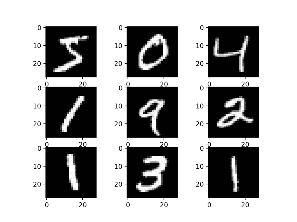
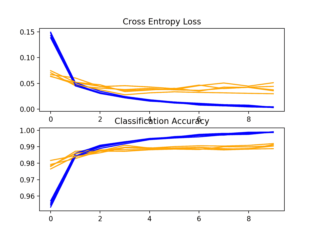
接下来，显示了一个诊断图，提供了对模型在每个折叠中的学习行为的洞察。

在这种情况下，我们可以看到该模型通常实现了良好的拟合，训练和测试学习曲线收敛。没有明显的过度或不足的迹象。

K 折交叉验证期间基线模型的损失和准确率学习曲线

接下来，计算模型表现的概要。

我们可以看到，在这种情况下，模型的估计技能约为 98.6%，这是合理的。

Accuracy: mean=98.677 std=0.107, n=5

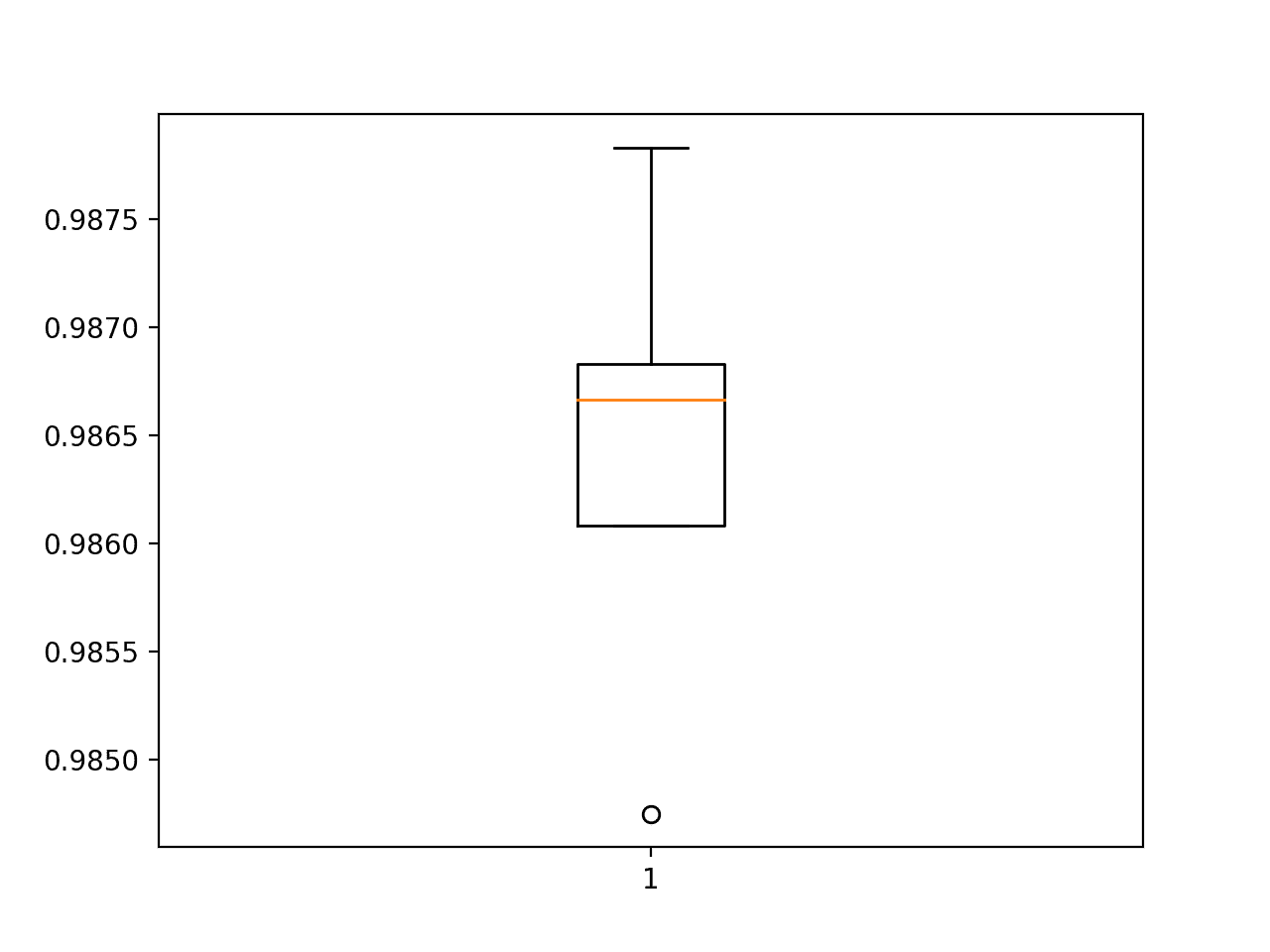
最后，创建一个方框和触须图来总结准确度分数的分布。

使用 k 倍交叉验证评估的基线模型准确度分数的方框图和须图

我们现在有了一个健壮的测试工具和一个表现良好的基线模型。

如何开发改进的模型

我们有很多方法可以探索基线模型的改进。

我们将关注模型配置中经常导致改进的领域，即所谓的低挂果实。第一个是学习算法的改变，第二个是模型深度的增加。

学习的改进

学习算法有许多方面可以探索改进。

也许最大的杠杆作用点是学习率，例如评估学习率的较小或较大值可能产生的影响，以及在培训期间改变学习率的时间表。

另一种可以快速加速模型学习并导致表现大幅提升的方法是批处理规范化。我们将评估批量标准化对基线模型的影响。

批量归一化可以在卷积层和全连通层之后使用。它具有改变层的输出分布的效果，特别是通过标准化输出。这具有稳定和加速学习过程的效果。

我们可以更新模型定义，以便在基线模型的卷积层和密集层的激活函数之后使用批处理规范化。带批量规格化的 define_model() 函数的更新版本如下。

# define cnn model
def define_model():
	model = Sequential()
	model.add(Conv2D(32, (3, 3), activation='relu', kernel_initializer='he_uniform', input_shape=(28, 28, 1)))
	model.add(BatchNormalization())
	model.add(MaxPooling2D((2, 2)))
	model.add(Flatten())
	model.add(Dense(100, activation='relu', kernel_initializer='he_uniform'))
	model.add(BatchNormalization())
	model.add(Dense(10, activation='softmax'))
	# compile model
	opt = SGD(learning_rate=0.01, momentum=0.9)
	model.compile(optimizer=opt, loss='categorical_crossentropy', metrics=['accuracy'])
	return model

下面提供了包含此更改的完整代码列表。

# cnn model with batch normalization for mnist
from numpy import mean
from numpy import std
from matplotlib import pyplot as plt
from sklearn.model_selection import KFold
from tensorflow.keras.datasets import mnist
from tensorflow.keras.utils import to_categorical
from tensorflow.keras.models import Sequential
from tensorflow.keras.layers import Conv2D
from tensorflow.keras.layers import MaxPooling2D
from tensorflow.keras.layers import Dense
from tensorflow.keras.layers import Flatten
from tensorflow.keras.optimizers import SGD
from tensorflow.keras.layers import BatchNormalization

# load train and test dataset
def load_dataset():
	# load dataset
	(trainX, trainY), (testX, testY) = mnist.load_data()
	# reshape dataset to have a single channel
	trainX = trainX.reshape((trainX.shape[0], 28, 28, 1))
	testX = testX.reshape((testX.shape[0], 28, 28, 1))
	# one hot encode target values
	trainY = to_categorical(trainY)
	testY = to_categorical(testY)
	return trainX, trainY, testX, testY

# scale pixels
def prep_pixels(train, test):
	# convert from integers to floats
	train_norm = train.astype('float32')
	test_norm = test.astype('float32')
	# normalize to range 0-1
	train_norm = train_norm / 255.0
	test_norm = test_norm / 255.0
	# return normalized images
	return train_norm, test_norm

# define cnn model
def define_model():
	model = Sequential()
	model.add(Conv2D(32, (3, 3), activation='relu', kernel_initializer='he_uniform', input_shape=(28, 28, 1)))
	model.add(BatchNormalization())
	model.add(MaxPooling2D((2, 2)))
	model.add(Flatten())
	model.add(Dense(100, activation='relu', kernel_initializer='he_uniform'))
	model.add(BatchNormalization())
	model.add(Dense(10, activation='softmax'))
	# compile model
	opt = SGD(learning_rate=0.01, momentum=0.9)
	model.compile(optimizer=opt, loss='categorical_crossentropy', metrics=['accuracy'])
	return model

# evaluate a model using k-fold cross-validation
def evaluate_model(dataX, dataY, n_folds=5):
	scores, histories = list(), list()
	# prepare cross validation
	kfold = KFold(n_folds, shuffle=True, random_state=1)
	# enumerate splits
	for train_ix, test_ix in kfold.split(dataX):
		# define model
		model = define_model()
		# select rows for train and test
		trainX, trainY, testX, testY = dataX[train_ix], dataY[train_ix], dataX[test_ix], dataY[test_ix]
		# fit model
		history = model.fit(trainX, trainY, epochs=10, batch_size=32, validation_data=(testX, testY), verbose=0)
		# evaluate model
		_, acc = model.evaluate(testX, testY, verbose=0)
		print('> %.3f' % (acc * 100.0))
		# stores scores
		scores.append(acc)
		histories.append(history)
	return scores, histories

# plot diagnostic learning curves
def summarize_diagnostics(histories):
	for i in range(len(histories)):
		# plot loss
		plt.subplot(2, 1, 1)
		plt.title('Cross Entropy Loss')
		plt.plot(histories[i].history['loss'], color='blue', label='train')
		plt.plot(histories[i].history['val_loss'], color='orange', label='test')
		# plot accuracy
		plt.subplot(2, 1, 2)
		plt.title('Classification Accuracy')
		plt.plot(histories[i].history['accuracy'], color='blue', label='train')
		plt.plot(histories[i].history['val_accuracy'], color='orange', label='test')
	plt.show()

# summarize model performance
def summarize_performance(scores):
	# print summary
	print('Accuracy: mean=%.3f std=%.3f, n=%d' % (mean(scores)*100, std(scores)*100, len(scores)))
	# box and whisker plots of results
	plt.boxplot(scores)
	plt.show()

# run the test harness for evaluating a model
def run_test_harness():
	# load dataset
	trainX, trainY, testX, testY = load_dataset()
	# prepare pixel data
	trainX, testX = prep_pixels(trainX, testX)
	# evaluate model
	scores, histories = evaluate_model(trainX, trainY)
	# learning curves
	summarize_diagnostics(histories)
	# summarize estimated performance
	summarize_performance(scores)

# entry point, run the test harness
run_test_harness()

再次运行该示例会报告交叉验证过程中每个折叠的模型表现。

注:考虑到算法或评估程序的随机性，或数值准确率的差异，您的结果可能会有所不同。考虑运行该示例几次，并比较平均结果。

与交叉验证折叠中的基线相比，我们可能会看到模型表现的小幅下降。

> 98.475
> 98.608
> 98.683
> 98.783
> 98.667

创建学习曲线的图，在这种情况下显示学习速度(相对于时代的改进)似乎与基线模型没有不同。

这些图表明，批量标准化，至少在这种情况下实现，不会带来任何好处。

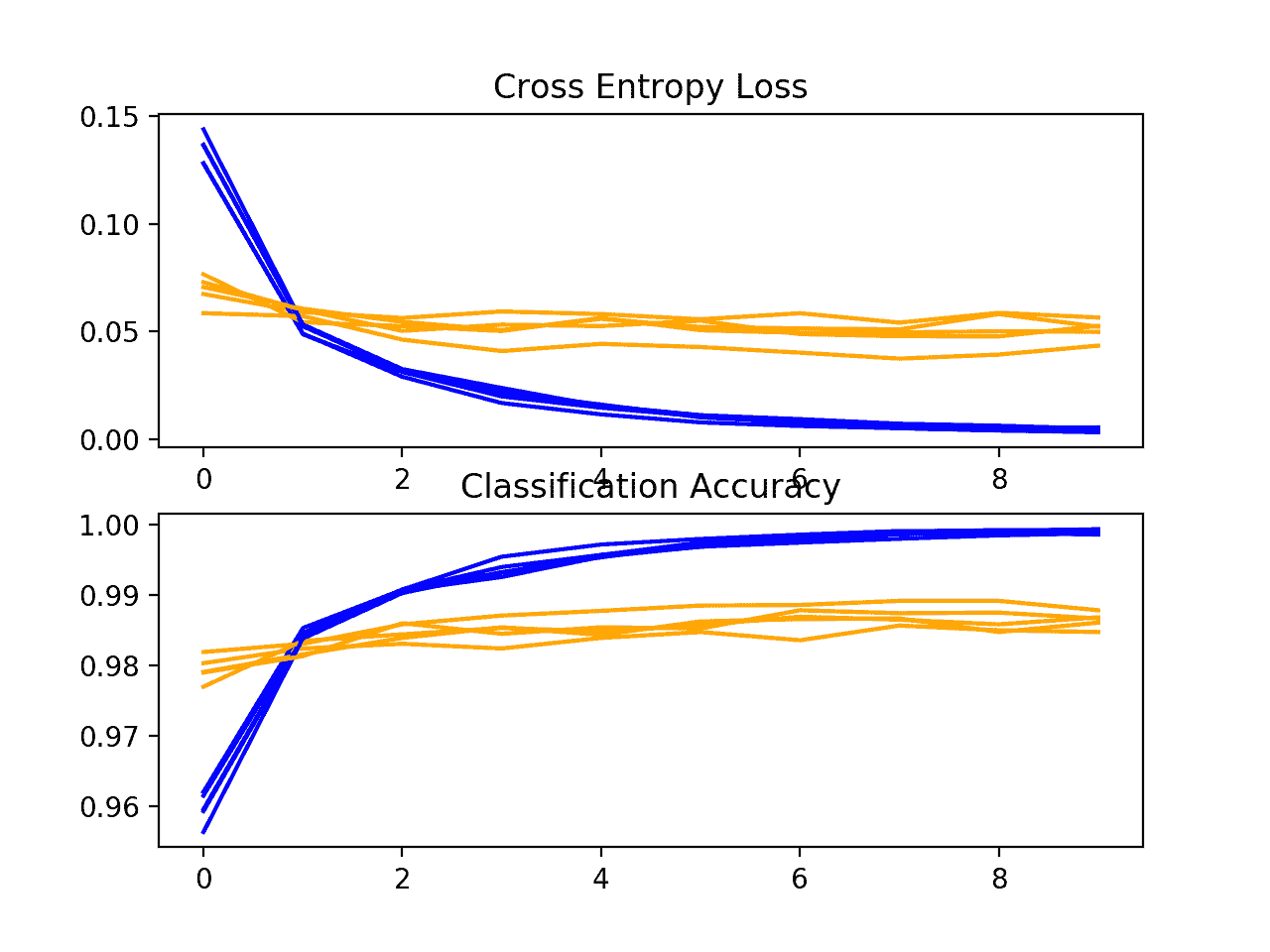
K 折交叉验证中批处理模型的损失和准确率学习曲线

接下来，给出了模型的估计表现，显示了模型的平均准确率略有下降的表现:与基线模型的 98.677 相比，为 98.643。

Accuracy: mean=98.643 std=0.101, n=5

使用 k 倍交叉验证评估的 BatchNormalization 模型的准确度分数的方框图和须图

模型深度增加

有许多方法可以改变模型配置，以探索对基线模型的改进。

两种常见的方法涉及改变模型的特征提取部分的容量或者改变模型的分类器部分的容量或功能。也许最大的影响点是对特征提取器的改变。

我们可以增加模型的特征提取器部分的深度，遵循类似 VGG 的模式，用相同大小的滤波器增加更多的卷积和池化层，同时增加滤波器的数量。在这种情况下，我们将添加一个双卷积层，每个层有 64 个滤波器，然后是另一个最大池层。

带有此更改的 define_model() 函数的更新版本如下所示。

# define cnn model
def define_model():
	model = Sequential()
	model.add(Conv2D(32, (3, 3), activation='relu', kernel_initializer='he_uniform', input_shape=(28, 28, 1)))
	model.add(MaxPooling2D((2, 2)))
	model.add(Conv2D(64, (3, 3), activation='relu', kernel_initializer='he_uniform'))
	model.add(Conv2D(64, (3, 3), activation='relu', kernel_initializer='he_uniform'))
	model.add(MaxPooling2D((2, 2)))
	model.add(Flatten())
	model.add(Dense(100, activation='relu', kernel_initializer='he_uniform'))
	model.add(Dense(10, activation='softmax'))
	# compile model
	opt = SGD(learning_rate=0.01, momentum=0.9)
	model.compile(optimizer=opt, loss='categorical_crossentropy', metrics=['accuracy'])
	return model

为了完整起见，下面提供了整个代码列表，包括这一更改。

# deeper cnn model for mnist
from numpy import mean
from numpy import std
from matplotlib import pyplot as plt
from sklearn.model_selection import KFold
from tensorflow.keras.datasets import mnist
from tensorflow.keras.utils import to_categorical
from tensorflow.keras.models import Sequential
from tensorflow.keras.layers import Conv2D
from tensorflow.keras.layers import MaxPooling2D
from tensorflow.keras.layers import Dense
from tensorflow.keras.layers import Flatten
from tensorflow.keras.optimizers import SGD

# load train and test dataset
def load_dataset():
	# load dataset
	(trainX, trainY), (testX, testY) = mnist.load_data()
	# reshape dataset to have a single channel
	trainX = trainX.reshape((trainX.shape[0], 28, 28, 1))
	testX = testX.reshape((testX.shape[0], 28, 28, 1))
	# one hot encode target values
	trainY = to_categorical(trainY)
	testY = to_categorical(testY)
	return trainX, trainY, testX, testY

# scale pixels
def prep_pixels(train, test):
	# convert from integers to floats
	train_norm = train.astype('float32')
	test_norm = test.astype('float32')
	# normalize to range 0-1
	train_norm = train_norm / 255.0
	test_norm = test_norm / 255.0
	# return normalized images
	return train_norm, test_norm

# define cnn model
def define_model():
	model = Sequential()
	model.add(Conv2D(32, (3, 3), activation='relu', kernel_initializer='he_uniform', input_shape=(28, 28, 1)))
	model.add(MaxPooling2D((2, 2)))
	model.add(Conv2D(64, (3, 3), activation='relu', kernel_initializer='he_uniform'))
	model.add(Conv2D(64, (3, 3), activation='relu', kernel_initializer='he_uniform'))
	model.add(MaxPooling2D((2, 2)))
	model.add(Flatten())
	model.add(Dense(100, activation='relu', kernel_initializer='he_uniform'))
	model.add(Dense(10, activation='softmax'))
	# compile model
	opt = SGD(learning_rate=0.01, momentum=0.9)
	model.compile(optimizer=opt, loss='categorical_crossentropy', metrics=['accuracy'])
	return model

# evaluate a model using k-fold cross-validation
def evaluate_model(dataX, dataY, n_folds=5):
	scores, histories = list(), list()
	# prepare cross validation
	kfold = KFold(n_folds, shuffle=True, random_state=1)
	# enumerate splits
	for train_ix, test_ix in kfold.split(dataX):
		# define model
		model = define_model()
		# select rows for train and test
		trainX, trainY, testX, testY = dataX[train_ix], dataY[train_ix], dataX[test_ix], dataY[test_ix]
		# fit model
		history = model.fit(trainX, trainY, epochs=10, batch_size=32, validation_data=(testX, testY), verbose=0)
		# evaluate model
		_, acc = model.evaluate(testX, testY, verbose=0)
		print('> %.3f' % (acc * 100.0))
		# stores scores
		scores.append(acc)
		histories.append(history)
	return scores, histories

# plot diagnostic learning curves
def summarize_diagnostics(histories):
	for i in range(len(histories)):
		# plot loss
		plt.subplot(2, 1, 1)
		plt.title('Cross Entropy Loss')
		plt.plot(histories[i].history['loss'], color='blue', label='train')
		plt.plot(histories[i].history['val_loss'], color='orange', label='test')
		# plot accuracy
		plt.subplot(2, 1, 2)
		plt.title('Classification Accuracy')
		plt.plot(histories[i].history['accuracy'], color='blue', label='train')
		plt.plot(histories[i].history['val_accuracy'], color='orange', label='test')
	plt.show()

# summarize model performance
def summarize_performance(scores):
	# print summary
	print('Accuracy: mean=%.3f std=%.3f, n=%d' % (mean(scores)*100, std(scores)*100, len(scores)))
	# box and whisker plots of results
	plt.boxplot(scores)
	plt.show()

# run the test harness for evaluating a model
def run_test_harness():
	# load dataset
	trainX, trainY, testX, testY = load_dataset()
	# prepare pixel data
	trainX, testX = prep_pixels(trainX, testX)
	# evaluate model
	scores, histories = evaluate_model(trainX, trainY)
	# learning curves
	summarize_diagnostics(histories)
	# summarize estimated performance
	summarize_performance(scores)

# entry point, run the test harness
run_test_harness()

运行该示例会报告交叉验证过程中每个折叠的模型表现。

注:考虑到算法或评估程序的随机性，或数值准确率的差异，您的结果可能会有所不同。考虑运行该示例几次，并比较平均结果。

每倍得分可能表明比基线有所改善。

> 99.058
> 99.042
> 98.883
> 99.192
> 99.133

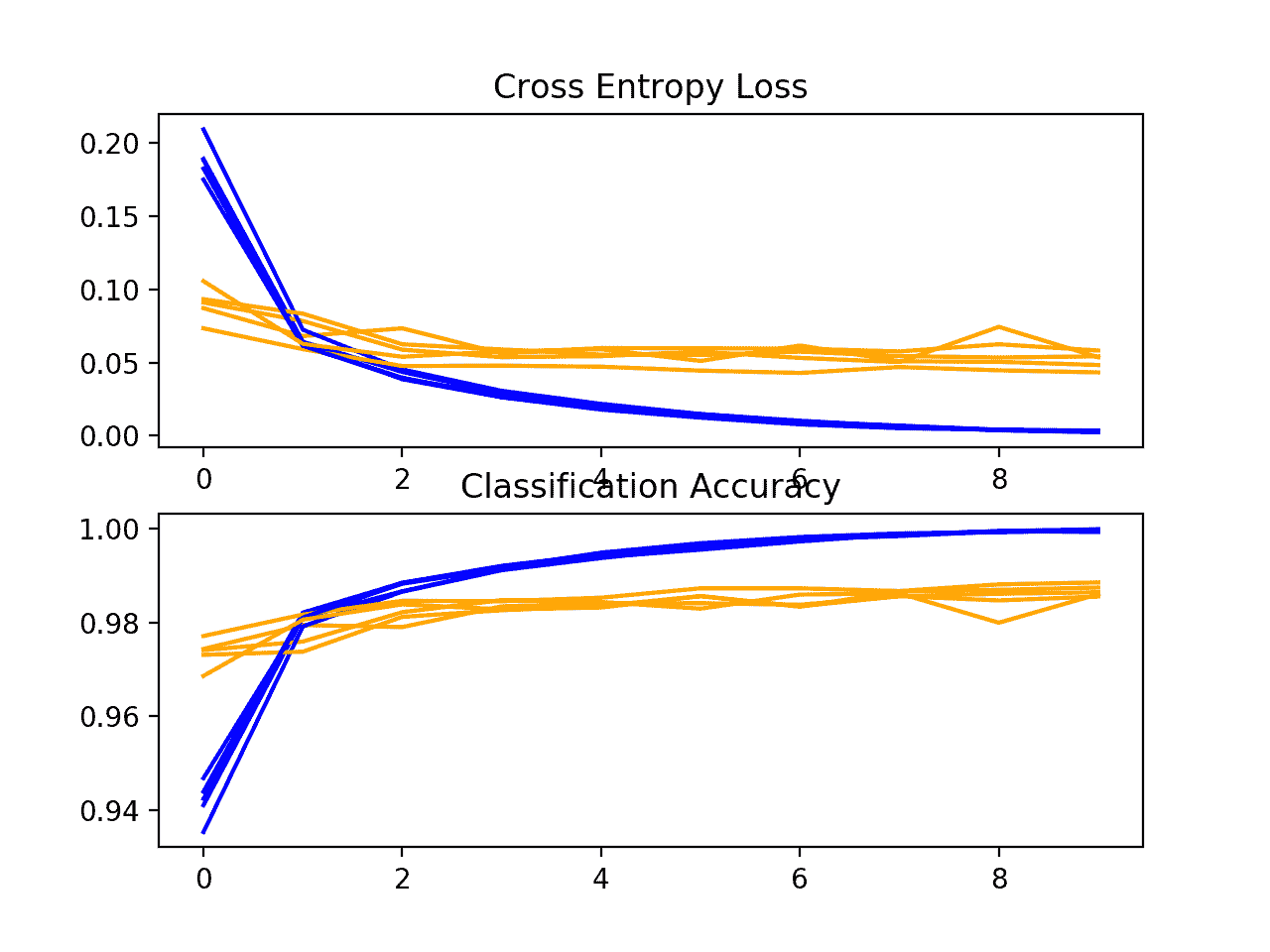
创建了一个学习曲线图，在这种情况下显示模型仍然很好地适合问题，没有明显的过拟合迹象。这些情节甚至表明，进一步的训练时期可能会有所帮助。

K 折交叉验证期间更深模型的损失和准确率学习曲线

接下来，给出了模型的估计表现，与基线相比，表现略有提高，从 98.677 提高到 99.062，标准偏差也略有下降。

Accuracy: mean=99.062 std=0.104, n=5

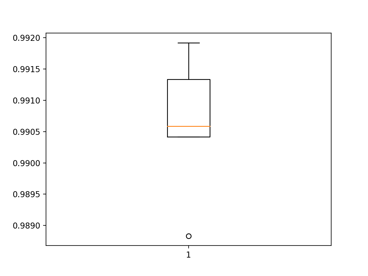
使用 k 倍交叉验证评估的更深模型的准确度分数的方框图和须图

如何最终确定模型并做出预测

只要我们有想法，有时间和资源来测试，模型改进的过程可能会持续很长时间。

在某些时候，必须选择并采用最终的模型配置。在这种情况下，我们将选择更深的模型作为最终模型。

首先，我们将最终确定我们的模型，但是在整个训练数据集上拟合一个模型，并将该模型保存到文件中供以后使用。然后，我们将加载模型，并在等待测试数据集上评估其表现，以了解所选模型在实践中的实际表现。最后，我们将使用保存的模型对单个图像进行预测。

保存最终模型

最终模型通常适合所有可用数据，例如所有训练和测试数据集的组合。

在本教程中，我们有意保留一个测试数据集，以便我们可以估计最终模型的表现，这在实践中可能是一个好主意。因此，我们将只在训练数据集上拟合我们的模型。

# fit model
model.fit(trainX, trainY, epochs=10, batch_size=32, verbose=0)

一旦合适，我们可以通过调用模型上的 save() 函数将最终模型保存到一个 H5 文件中，并传入选择的文件名。

# save model
model.save('final_model.h5')

注意，保存和加载 Keras 模型需要在您的工作站上安装 h5py 库。

下面列出了在训练数据集上拟合最终深度模型并将其保存到文件中的完整示例。

# save the final model to file
from tensorflow.keras.datasets import mnist
from tensorflow.keras.utils import to_categorical
from tensorflow.keras.models import Sequential
from tensorflow.keras.layers import Conv2D
from tensorflow.keras.layers import MaxPooling2D
from tensorflow.keras.layers import Dense
from tensorflow.keras.layers import Flatten
from tensorflow.keras.optimizers import SGD

# load train and test dataset
def load_dataset():
	# load dataset
	(trainX, trainY), (testX, testY) = mnist.load_data()
	# reshape dataset to have a single channel
	trainX = trainX.reshape((trainX.shape[0], 28, 28, 1))
	testX = testX.reshape((testX.shape[0], 28, 28, 1))
	# one hot encode target values
	trainY = to_categorical(trainY)
	testY = to_categorical(testY)
	return trainX, trainY, testX, testY

# scale pixels
def prep_pixels(train, test):
	# convert from integers to floats
	train_norm = train.astype('float32')
	test_norm = test.astype('float32')
	# normalize to range 0-1
	train_norm = train_norm / 255.0
	test_norm = test_norm / 255.0
	# return normalized images
	return train_norm, test_norm

# define cnn model
def define_model():
	model = Sequential()
	model.add(Conv2D(32, (3, 3), activation='relu', kernel_initializer='he_uniform', input_shape=(28, 28, 1)))
	model.add(MaxPooling2D((2, 2)))
	model.add(Conv2D(64, (3, 3), activation='relu', kernel_initializer='he_uniform'))
	model.add(Conv2D(64, (3, 3), activation='relu', kernel_initializer='he_uniform'))
	model.add(MaxPooling2D((2, 2)))
	model.add(Flatten())
	model.add(Dense(100, activation='relu', kernel_initializer='he_uniform'))
	model.add(Dense(10, activation='softmax'))
	# compile model
	opt = SGD(learning_rate=0.01, momentum=0.9)
	model.compile(optimizer=opt, loss='categorical_crossentropy', metrics=['accuracy'])
	return model

# run the test harness for evaluating a model
def run_test_harness():
	# load dataset
	trainX, trainY, testX, testY = load_dataset()
	# prepare pixel data
	trainX, testX = prep_pixels(trainX, testX)
	# define model
	model = define_model()
	# fit model
	model.fit(trainX, trainY, epochs=10, batch_size=32, verbose=0)
	# save model
	model.save('final_model.h5')

# entry point, run the test harness
run_test_harness()

运行此示例后，您将在当前工作目录中拥有一个名为“ final_model.h5 ”的 1.2 兆字节文件。

评估最终模型

我们现在可以加载最终模型，并在等待测试数据集上对其进行评估。

如果我们有兴趣向项目涉众展示所选模型的表现，这是我们可以做的事情。

可通过 load_model() 功能加载模型。

下面列出了加载保存的模型并在测试数据集上对其进行评估的完整示例。

# evaluate the deep model on the test dataset
from tensorflow.keras.datasets import mnist
from tensorflow.keras.models import load_model
from tensorflow.keras.utils import to_categorical

# load train and test dataset
def load_dataset():
	# load dataset
	(trainX, trainY), (testX, testY) = mnist.load_data()
	# reshape dataset to have a single channel
	trainX = trainX.reshape((trainX.shape[0], 28, 28, 1))
	testX = testX.reshape((testX.shape[0], 28, 28, 1))
	# one hot encode target values
	trainY = to_categorical(trainY)
	testY = to_categorical(testY)
	return trainX, trainY, testX, testY

# scale pixels
def prep_pixels(train, test):
	# convert from integers to floats
	train_norm = train.astype('float32')
	test_norm = test.astype('float32')
	# normalize to range 0-1
	train_norm = train_norm / 255.0
	test_norm = test_norm / 255.0
	# return normalized images
	return train_norm, test_norm

# run the test harness for evaluating a model
def run_test_harness():
	# load dataset
	trainX, trainY, testX, testY = load_dataset()
	# prepare pixel data
	trainX, testX = prep_pixels(trainX, testX)
	# load model
	model = load_model('final_model.h5')
	# evaluate model on test dataset
	_, acc = model.evaluate(testX, testY, verbose=0)
	print('> %.3f' % (acc * 100.0))

# entry point, run the test harness
run_test_harness()

运行该示例将加载保存的模型，并在暂挂测试数据集上评估该模型。

注:考虑到算法或评估程序的随机性，或数值准确率的差异，您的结果可能会有所不同。考虑运行该示例几次，并比较平均结果。

计算并打印测试数据集中模型的分类准确率。在这种情况下，我们可以看到该模型达到了 99.090%的准确率，或者仅仅不到 1%，这一点也不差，并且相当接近估计的 99.753%，标准偏差约为 0.5%(例如 99%的分数)。

> 99.090

作出预测

我们可以使用保存的模型对新图像进行预测。

该模型假设新图像是灰度级的，它们已经对齐，使得一个图像包含一个居中的手写数字，并且图像的大小是 28×28 像素的正方形。

下面是从 MNIST 测试数据集中提取的图像。您可以将其保存在当前工作目录中，文件名为“ sample_image.png ”。

示例手写数字

• 下载样本图像(sample_image.png)

我们将假设这是一个全新的、看不见的图像，以所需的方式准备，并看看我们如何使用保存的模型来预测图像所代表的整数(例如，我们期望“ 7 ”)。

首先，我们可以加载图像，强制为灰度格式，并强制大小为 28×28 像素。然后，可以调整加载图像的大小，使其具有单个通道，并表示数据集中的单个样本。 load_image() 函数实现了这一点，并将返回已加载的准备分类的图像。

重要的是，像素值的准备方式与在拟合最终模型时为训练数据集准备像素值的方式相同，在这种情况下，最终模型是归一化的。

# load and prepare the image
def load_image(filename):
	# load the image
	img = load_img(filename, grayscale=True, target_size=(28, 28))
	# convert to array
	img = img_to_array(img)
	# reshape into a single sample with 1 channel
	img = img.reshape(1, 28, 28, 1)
	# prepare pixel data
	img = img.astype('float32')
	img = img / 255.0
	return img

接下来，我们可以像上一节一样加载模型，调用 predict() 函数得到预测得分，然后使用 argmax() 得到图像所代表的数字。

# predict the class
predict_value = model.predict(img)
digit = argmax(predict_value)

下面列出了完整的示例。

# make a prediction for a new image.
from numpy import argmax
from keras.preprocessing.image import load_img
from keras.preprocessing.image import img_to_array
from keras.models import load_model

# load and prepare the image
def load_image(filename):
	# load the image
	img = load_img(filename, grayscale=True, target_size=(28, 28))
	# convert to array
	img = img_to_array(img)
	# reshape into a single sample with 1 channel
	img = img.reshape(1, 28, 28, 1)
	# prepare pixel data
	img = img.astype('float32')
	img = img / 255.0
	return img

# load an image and predict the class
def run_example():
	# load the image
	img = load_image('sample_image.png')
	# load model
	model = load_model('final_model.h5')
	# predict the class
	predict_value = model.predict(img)
	digit = argmax(predict_value)
	print(digit)

# entry point, run the example
run_example()

运行该示例首先加载和准备图像，加载模型，然后正确预测加载的图像代表数字“ 7 ”。

7

扩展ˌ扩张

本节列出了一些您可能希望探索的扩展教程的想法。

• 调整像素缩放。探索与基线模型相比，替代像素缩放方法如何影响模型表现，包括居中和标准化。
• 调整学习率。探究与基线模型相比，不同的学习率如何影响模型表现，例如 0.001 和 0.0001。
• 调整模型深度。探索与基线模型相比，向模型中添加更多层如何影响模型表现，例如模型的分类器部分中的另一个卷积和池层块或另一个密集层。

如果你探索这些扩展，我很想知道。
在下面的评论中发表你的发现。

进一步阅读

如果您想更深入地了解这个主题，本节将提供更多资源。

蜜蜂

• 硬数据集 API
• Keras 数据集代码
• sklearn.model_selection。KFold 原料药

文章

• MNIST 数据库，维基百科。
• 类别数据集结果，这个图像的类别是什么？

摘要

在本教程中，您发现了如何从零开始开发用于手写数字分类的卷积神经网络。

具体来说，您了解到:

• 如何开发一个测试工具来开发一个健壮的模型评估，并为分类任务建立一个表现基线。
• 如何探索基线模型的扩展，以提高学习和模型能力。
• 如何开发最终模型，评估最终模型的表现，并使用它对新图像进行预测。

你有什么问题吗？
在下面的评论中提问，我会尽力回答。

如何分类猫狗照片（准确率 97%）

原文：https://machinelearningmastery.com/how-to-develop-a-convolutional-neural-network-to-classify-photos-of-dogs-and-cats/

最后更新于 2021 年 12 月 8 日

逐步开发深度卷积神经网络对狗和猫的照片进行分类

狗与猫数据集是一个标准的计算机视觉数据集，包括将照片分类为包含狗或猫。

虽然这个问题听起来很简单，但它只是在过去几年中使用深度学习卷积神经网络得到了有效解决。在数据集得到有效解决的同时，它可以作为学习和实践如何从零开始开发、评估和使用卷积深度学习神经网络进行图像分类的基础。

这包括如何开发一个健壮的测试工具来评估模型的表现，如何探索模型的改进，以及如何保存模型并在以后加载它来对新数据进行预测。

在本教程中，您将发现如何开发一个卷积神经网络来对狗和猫的照片进行分类。

完成本教程后，您将知道:

• 如何加载和准备狗和猫的照片进行建模？
• 如何从零开始开发卷积神经网络进行照片分类并提高模型表现？
• 如何利用迁移学习开发照片分类模型？

用我的新书计算机视觉深度学习启动你的项目，包括分步教程和所有示例的 Python 源代码文件。

我们开始吧。

• 2019 年 10 月更新:针对 Keras 2.3 和 TensorFlow 2.0 更新。
• 2021 年 12 月更新:修复“预处理照片尺寸(可选)”部分代码中的错别字

如何开发卷积神经网络来对狗和猫的照片进行分类
照片作者:科恩·范德维尔德，版权所有。

教程概述

本教程分为六个部分；它们是:

1. 狗与猫的预测问题
2. 狗与猫数据集准备
3. 开发一个基线有线电视新闻网模型
4. 开发模型改进
5. 探索迁移学习
6. 如何最终确定模型并做出预测

狗与猫的预测问题

狗 vs 猫数据集是指 2013 年举行的 Kaggle 机器学习竞赛中使用的数据集。

数据集由狗和猫的照片组成，这些照片是从 300 万张手动注释照片的更大数据集中提供的照片子集。该数据集是 Petfinder.com 和微软合作开发的。

该数据集最初被用作验证码(或完全自动的公共图灵测试，以区分计算机和人类)，即一项被认为是人类发现微不足道但机器无法解决的任务，用于网站上区分人类用户和机器人。具体来说，该任务被称为“限制访问的动物物种图像识别”，这是验证码的一种。这项任务在 2007 年的论文《T2·阿西拉:利用兴趣对齐的手动图像分类的验证码》中有所描述。

我们展示了阿西拉，一种验证码，要求用户从一组 12 张猫和狗的照片中识别猫。Asirra 对用户来说很容易；用户研究表明，人类可以在 30 秒内解决 99.6%的问题。除非机器视觉取得重大进展，否则我们预计计算机解决这个问题的可能性不会超过 1/54，000。

——Asirra:利用兴趣对齐的手动图像分类的验证码，2007。

在比赛发布时，最先进的结果是通过一个 SVM 实现的，并在 2007 年的一篇论文中进行了描述，该论文的标题为“对阿西拉验证码的机器学习攻击”(PDF)达到了 80%的分类准确率。正是这篇论文证明了在任务被提出后不久，该任务就不再是适合验证码的任务。

……我们描述了一个分类器，它在区分在 Asirra 中使用的猫和狗的图像方面有 82.7%的准确性。该分类器是基于从图像中提取的颜色和纹理特征训练的支持向量机分类器的组合。[……]我们的结果表明，不要在没有保障措施的情况下部署阿西拉。

——针对 Asirra 验证码的机器学习攻击，2007 年。

卡格尔竞赛提供了 25000 张贴有标签的照片:12500 只狗和同样数量的猫。然后需要对 12，500 张未标记照片的测试数据集进行预测。比赛由皮埃尔·塞马奈(目前是谷歌大脑的一名研究科学家)赢得，他在 70%的测试数据集子样本上获得了大约 98.914%的分类准确率。他的方法后来被描述为 2013 年论文的一部分，题为“T2 超吃:使用卷积网络的集成识别、定位和检测”

数据集很容易理解，并且小到可以放入内存。因此，当初学者开始使用卷积神经网络时，它已经成为一个很好的“你好世界”或“入门”计算机视觉数据集。

因此，在此任务中，使用手动设计的卷积神经网络达到大约 80%的准确率和使用转移学习达到 90%+的准确率是常规的。

狗与猫数据集准备

数据集可以从 Kaggle 网站免费下载，虽然我相信你一定有 Kaggle 账号。

如果您没有 Kaggle 帐户，请先注册。

通过访问犬猫数据页面下载数据集，点击全部下载按钮。

这会将 850 兆字节的文件“ dogs-vs-cats.zip ”下载到你的工作站。

解压文件，你会看到列车. zip 、列车 1.zip 和一个*。csv* 文件。解压缩 train.zip 文件，因为我们将只关注这个数据集。

现在，您将拥有一个名为“ train/ ”的文件夹，其中包含 25，000 个。狗和猫的 jpg 文件。这些照片是用它们的文件名标注的，带有“T2”狗“T3”或“T4”猫“T5”的字样。文件命名约定如下:

cat.0.jpg
...
cat.124999.jpg
dog.0.jpg
dog.124999.jpg

绘制狗和猫的照片

在目录里随便看几张照片，可以看到照片是彩色的，形状大小不一。

例如，让我们将狗的前九张照片加载并绘制成一个图形。

下面列出了完整的示例。

# plot dog photos from the dogs vs cats dataset
from matplotlib import pyplot
from matplotlib.image import imread
# define location of dataset
folder = 'train/'
# plot first few images
for i in range(9):
	# define subplot
	pyplot.subplot(330 + 1 + i)
	# define filename
	filename = folder + 'dog.' + str(i) + '.jpg'
	# load image pixels
	image = imread(filename)
	# plot raw pixel data
	pyplot.imshow(image)
# show the figure
pyplot.show()

运行该示例会创建一个图表，显示数据集中狗的前九张照片。

我们可以看到有些照片是风景格式的，有些是人像格式的，有些是方形的。

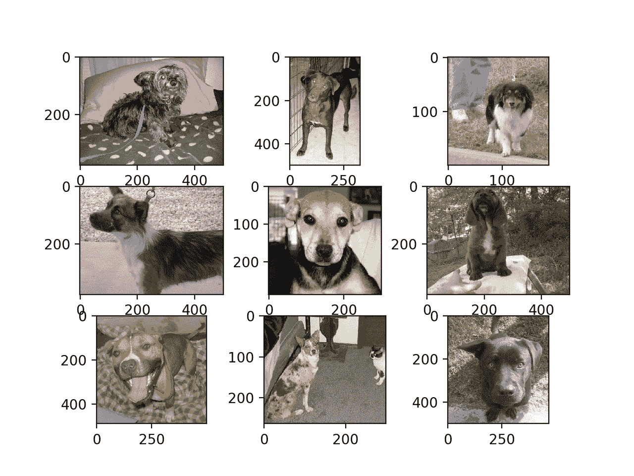
狗与猫数据集中狗的前九张照片图

我们可以更新示例，改为绘制猫咪照片；下面列出了完整的示例。

# plot cat photos from the dogs vs cats dataset
from matplotlib import pyplot
from matplotlib.image import imread
# define location of dataset
folder = 'train/'
# plot first few images
for i in range(9):
	# define subplot
	pyplot.subplot(330 + 1 + i)
	# define filename
	filename = folder + 'cat.' + str(i) + '.jpg'
	# load image pixels
	image = imread(filename)
	# plot raw pixel data
	pyplot.imshow(image)
# show the figure
pyplot.show()

同样，我们可以看到照片都是不同的尺寸。

我们还可以看到一张猫几乎看不见的照片(左下角)和另一张有两只猫的照片(右下角)。这表明任何适合这个问题的分类器都必须是健壮的。

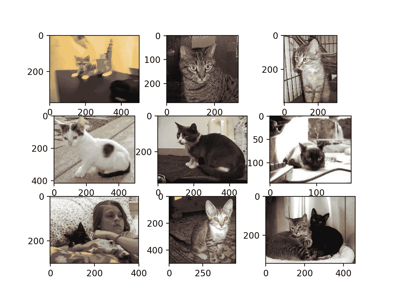
狗与猫数据集中猫的前九张照片图

选择标准化照片尺寸

这些照片必须在建模前进行重塑，以便所有图像具有相同的形状。这通常是一个小正方形图像。

有许多方法可以实现这一点，尽管最常见的是一个简单的调整大小操作，它将拉伸和变形每个图像的纵横比，并强制将其转换为新的形状。

我们可以加载所有照片，查看照片宽度和高度的分布，然后设计一个新的照片大小，最好地反映我们在实践中最有可能看到的内容。

较小的输入意味着模型的训练速度更快，通常这种考虑主导了图像尺寸的选择。在这种情况下，我们将遵循这种方法，选择 200×200 像素的固定大小。

预处理照片尺寸(可选)

如果我们想将所有图像加载到内存中，我们可以估计它需要大约 12gb 的内存。

即 25，000 幅图像，每幅图像 200x200x3 像素，即 3，000，000，000 个 32 位像素值。

我们可以加载所有的图像，重塑它们，并将它们存储为一个 NumPy 数组。这可以放入许多现代机器的内存中，但不是全部，尤其是如果你只有 8gb 的空间。

我们可以编写自定义代码将图像加载到内存中，并在加载过程中调整它们的大小，然后保存它们以备建模。

下面的示例使用 Keras 图像处理 API 加载训练数据集中的所有 25，000 张照片，并将其重塑为 200×200 平方的照片。标签也是根据文件名为每张照片确定的。然后保存一组照片和标签。

# load dogs vs cats dataset, reshape and save to a new file
from os import listdir
from numpy import asarray
from numpy import save
from keras.preprocessing.image import load_img
from keras.preprocessing.image import img_to_array
# define location of dataset
folder = 'train/'
photos, labels = list(), list()
# enumerate files in the directory
for file in listdir(folder):
	# determine class
	output = 0.0
	if file.startswith('dog'):
		output = 1.0
	# load image
	photo = load_img(folder + file, target_size=(200, 200))
	# convert to numpy array
	photo = img_to_array(photo)
	# store
	photos.append(photo)
	labels.append(output)
# convert to a numpy arrays
photos = asarray(photos)
labels = asarray(labels)
print(photos.shape, labels.shape)
# save the reshaped photos
save('dogs_vs_cats_photos.npy', photos)
save('dogs_vs_cats_labels.npy', labels)

运行该示例可能需要大约一分钟的时间将所有图像加载到内存中，并打印加载数据的形状，以确认其加载正确。

注意:运行这个例子假设你有超过 12gb 的内存。如果没有足够的内存，可以跳过这个例子；它仅作为演示提供。

(25000, 200, 200, 3) (25000,)

运行结束时，将创建两个名为“dogs _ vs _ cat _ photos . npy”和“dogs _ vs _ cat _ labels . npy的文件，其中包含所有调整大小的图像及其关联的类别标签。这些文件总共只有大约 12 千兆字节，加载速度比单个图像快得多。

准备好的数据可以直接加载；例如:

# load and confirm the shape
from numpy import load
photos = load('dogs_vs_cats_photos.npy')
labels = load('dogs_vs_cats_labels.npy')
print(photos.shape, labels.shape)

将照片预处理到标准目录中

或者，我们可以使用 Keras ImageDataGenerator 类和*flow _ from _ directory()*API 逐步加载图像。这将会降低执行速度，但会在更多的机器上运行。

该 API 更倾向于将数据划分为单独的 train/ 和 test/ 目录，并且在每个目录下为每个类都有一个子目录，例如一个 train/dog/ 和一个 train/cat/ 子目录，同样用于测试。然后，图像被组织在子目录下。

我们可以编写一个脚本来创建具有这种首选结构的数据集副本。我们将随机选择 25%的图像(或 6，250 张)用于测试数据集。

首先，我们需要创建如下目录结构:

dataset_dogs_vs_cats
├── test
│   ├── cats
│   └── dogs
└── train
    ├── cats
    └── dogs

我们可以使用 makedirs() 函数在 Python 中创建目录，并使用循环为 train/ 和 test/ 目录创建 dog/ 和 cat/ 子目录。

# create directories
dataset_home = 'dataset_dogs_vs_cats/'
subdirs = ['train/', 'test/']
for subdir in subdirs:
	# create label subdirectories
	labeldirs = ['dogs/', 'cats/']
	for labldir in labeldirs:
		newdir = dataset_home + subdir + labldir
		makedirs(newdir, exist_ok=True)

接下来，我们可以枚举数据集中的所有图像文件，并根据它们的文件名将其复制到狗/ 或猫/ 子目录中。

此外，我们可以随机决定将 25%的图像保留在测试数据集中。这是通过固定伪随机数发生器的种子来实现的，这样我们每次运行代码时都会得到相同的数据分割。

# seed random number generator
seed(1)
# define ratio of pictures to use for validation
val_ratio = 0.25
# copy training dataset images into subdirectories
src_directory = 'train/'
for file in listdir(src_directory):
	src = src_directory + '/' + file
	dst_dir = 'train/'
	if random() < val_ratio:
		dst_dir = 'test/'
	if file.startswith('cat'):
		dst = dataset_home + dst_dir + 'cats/'  + file
		copyfile(src, dst)
	elif file.startswith('dog'):
		dst = dataset_home + dst_dir + 'dogs/'  + file
		copyfile(src, dst)

下面列出了完整的代码示例，并假设您已经将下载的 train.zip 中的图像解压缩到了 train/ 中的当前工作目录中。

# organize dataset into a useful structure
from os import makedirs
from os import listdir
from shutil import copyfile
from random import seed
from random import random
# create directories
dataset_home = 'dataset_dogs_vs_cats/'
subdirs = ['train/', 'test/']
for subdir in subdirs:
	# create label subdirectories
	labeldirs = ['dogs/', 'cats/']
	for labldir in labeldirs:
		newdir = dataset_home + subdir + labldir
		makedirs(newdir, exist_ok=True)
# seed random number generator
seed(1)
# define ratio of pictures to use for validation
val_ratio = 0.25
# copy training dataset images into subdirectories
src_directory = 'train/'
for file in listdir(src_directory):
	src = src_directory + '/' + file
	dst_dir = 'train/'
	if random() < val_ratio:
		dst_dir = 'test/'
	if file.startswith('cat'):
		dst = dataset_home + dst_dir + 'cats/'  + file
		copyfile(src, dst)
	elif file.startswith('dog'):
		dst = dataset_home + dst_dir + 'dogs/'  + file
		copyfile(src, dst)

运行示例后，您现在将拥有一个新的*dataset _ dogs _ vs _ cat/目录，其中包含一个 train/ 和 val/ 子文件夹，此外 dogs/ 还可以包含cat/*子目录，与设计完全一致。

开发一个基线有线电视新闻网模型

在本节中，我们可以为狗和猫数据集开发一个基线卷积神经网络模型。

基线模型将建立一个最低的模型表现，我们所有的其他模型都可以与之进行比较，以及一个我们可以用作研究和改进基础的模型架构。

一个很好的起点是 VGG 模型的一般架构原则。这些是一个很好的起点，因为它们在 ILSVRC 2014 竞赛中取得了顶级的表现，并且因为体系结构的模块化结构易于理解和实现。有关 VGG 模型的更多详细信息，请参见 2015 年的论文“用于大规模图像识别的超深度卷积网络”

该架构包括堆叠卷积层和 3×3 小滤波器，然后是最大池层。这些层一起形成一个块，并且这些块可以重复，其中每个块中的过滤器的数量随着网络的深度而增加，例如对于模型的前四个块为 32、64、128、256。卷积层上使用填充，以确保输出要素图的高度和宽度形状与输入匹配。

我们可以在狗与猫的问题上探索这种体系结构，并将一个模型与具有 1、2 和 3 个块的这种体系结构进行比较。

每层将使用 ReLU 激活功能和 he 权重初始化，这通常是最佳实践。例如，一个 3 块 VGG 风格的体系结构，其中每个块都有一个卷积和池层，可以在 Keras 中定义如下:

# block 1
model.add(Conv2D(32, (3, 3), activation='relu', kernel_initializer='he_uniform', padding='same', input_shape=(200, 200, 3)))
model.add(MaxPooling2D((2, 2)))
# block 2
model.add(Conv2D(64, (3, 3), activation='relu', kernel_initializer='he_uniform', padding='same'))
model.add(MaxPooling2D((2, 2)))
# block 3
model.add(Conv2D(128, (3, 3), activation='relu', kernel_initializer='he_uniform', padding='same'))
model.add(MaxPooling2D((2, 2)))

我们可以创建一个名为 define_model() 的函数，该函数将定义一个模型，并将其返回以准备好适应数据集。然后可以定制该功能来定义不同的基线模型，例如，具有 1、2 或 3 个 VGG 风格块的模型版本。

该模型将适用于随机梯度下降，我们将从 0.001 的保守学习率和 0.9 的动量开始。

这个问题是一个二进制分类任务，需要预测一个 0 或 1 的值。将使用具有 1 个节点和 sigmoid 激活的输出层，并将使用二元交叉熵损失函数优化模型。

下面是 define_model() 函数的一个例子，该函数用一个 vgg 类型的块来定义狗对猫问题的卷积神经网络模型。

# define cnn model
def define_model():
	model = Sequential()
	model.add(Conv2D(32, (3, 3), activation='relu', kernel_initializer='he_uniform', padding='same', input_shape=(200, 200, 3)))
	model.add(MaxPooling2D((2, 2)))
	model.add(Flatten())
	model.add(Dense(128, activation='relu', kernel_initializer='he_uniform'))
	model.add(Dense(1, activation='sigmoid'))
	# compile model
	opt = SGD(lr=0.001, momentum=0.9)
	model.compile(optimizer=opt, loss='binary_crossentropy', metrics=['accuracy'])
	return model

可以根据需要调用它来准备模型，例如:

# define model
model = define_model()

接下来，我们需要准备数据。

这包括首先定义图像数据生成器的实例，该实例将像素值缩放到 0-1 的范围。

# create data generator
datagen = ImageDataGenerator(rescale=1.0/255.0)

接下来，需要为训练和测试数据集准备迭代器。

我们可以在数据生成器上使用 flow_from_directory() 函数，并为列车/ 和测试/ 目录各创建一个迭代器。我们必须通过“ class_mode ”参数指定问题为二值分类问题，并通过“ target_size ”参数加载 200×200 像素大小的图像。我们将把批量固定在 64。

# prepare iterators
train_it = datagen.flow_from_directory('dataset_dogs_vs_cats/train/',
	class_mode='binary', batch_size=64, target_size=(200, 200))
test_it = datagen.flow_from_directory('dataset_dogs_vs_cats/test/',
	class_mode='binary', batch_size=64, target_size=(200, 200))

然后，我们可以使用训练迭代器( train_it )拟合模型，并在训练期间使用测试迭代器( test_it )作为验证数据集。

必须指定训练和测试迭代器的步数。这是构成一个纪元的批次数量。这可以通过每个迭代器的长度来指定，并且将是训练和测试目录中的图像总数除以批次大小(64)。

该模型将适合 20 个时代，这是一个很小的数字，用于检查模型是否能够学习问题。

# fit model
history = model.fit_generator(train_it, steps_per_epoch=len(train_it),
	validation_data=test_it, validation_steps=len(test_it), epochs=20, verbose=0)

一旦拟合，最终模型可以直接在测试数据集上进行评估，并报告分类准确率。

# evaluate model
_, acc = model.evaluate_generator(test_it, steps=len(test_it), verbose=0)
print('> %.3f' % (acc * 100.0))

最后，我们可以创建一个存储在从调用 fit_generator() 返回的“ history ”目录中的训练期间收集的历史的图。

历史记录包含每个时期结束时测试和训练数据集的模型准确率和损失。这些度量在训练时期的线图提供了学习曲线，我们可以用它来了解模型是过拟合、欠拟合还是拟合良好。

下面的*summary _ diagnostics()*函数获取历史目录，并创建一个单独的数字，一个是损失的线图，另一个是准确率图。然后，图形被保存到一个文件中，该文件的文件名基于脚本的名称。如果我们希望评估不同文件中模型的许多变化，并为每个变化自动创建线图，这将非常有用。

# plot diagnostic learning curves
def summarize_diagnostics(history):
	# plot loss
	pyplot.subplot(211)
	pyplot.title('Cross Entropy Loss')
	pyplot.plot(history.history['loss'], color='blue', label='train')
	pyplot.plot(history.history['val_loss'], color='orange', label='test')
	# plot accuracy
	pyplot.subplot(212)
	pyplot.title('Classification Accuracy')
	pyplot.plot(history.history['accuracy'], color='blue', label='train')
	pyplot.plot(history.history['val_accuracy'], color='orange', label='test')
	# save plot to file
	filename = sys.argv[0].split('/')[-1]
	pyplot.savefig(filename + '_plot.png')
	pyplot.close()

我们可以将所有这些结合到一个简单的测试工具中，用于测试模型配置。

下面列出了在狗和猫数据集上评估单块基线模型的完整示例。

# baseline model for the dogs vs cats dataset
import sys
from matplotlib import pyplot
from keras.utils import to_categorical
from keras.models import Sequential
from keras.layers import Conv2D
from keras.layers import MaxPooling2D
from keras.layers import Dense
from keras.layers import Flatten
from keras.optimizers import SGD
from keras.preprocessing.image import ImageDataGenerator

# define cnn model
def define_model():
	model = Sequential()
	model.add(Conv2D(32, (3, 3), activation='relu', kernel_initializer='he_uniform', padding='same', input_shape=(200, 200, 3)))
	model.add(MaxPooling2D((2, 2)))
	model.add(Flatten())
	model.add(Dense(128, activation='relu', kernel_initializer='he_uniform'))
	model.add(Dense(1, activation='sigmoid'))
	# compile model
	opt = SGD(lr=0.001, momentum=0.9)
	model.compile(optimizer=opt, loss='binary_crossentropy', metrics=['accuracy'])
	return model

# plot diagnostic learning curves
def summarize_diagnostics(history):
	# plot loss
	pyplot.subplot(211)
	pyplot.title('Cross Entropy Loss')
	pyplot.plot(history.history['loss'], color='blue', label='train')
	pyplot.plot(history.history['val_loss'], color='orange', label='test')
	# plot accuracy
	pyplot.subplot(212)
	pyplot.title('Classification Accuracy')
	pyplot.plot(history.history['accuracy'], color='blue', label='train')
	pyplot.plot(history.history['val_accuracy'], color='orange', label='test')
	# save plot to file
	filename = sys.argv[0].split('/')[-1]
	pyplot.savefig(filename + '_plot.png')
	pyplot.close()

# run the test harness for evaluating a model
def run_test_harness():
	# define model
	model = define_model()
	# create data generator
	datagen = ImageDataGenerator(rescale=1.0/255.0)
	# prepare iterators
	train_it = datagen.flow_from_directory('dataset_dogs_vs_cats/train/',
		class_mode='binary', batch_size=64, target_size=(200, 200))
	test_it = datagen.flow_from_directory('dataset_dogs_vs_cats/test/',
		class_mode='binary', batch_size=64, target_size=(200, 200))
	# fit model
	history = model.fit_generator(train_it, steps_per_epoch=len(train_it),
		validation_data=test_it, validation_steps=len(test_it), epochs=20, verbose=0)
	# evaluate model
	_, acc = model.evaluate_generator(test_it, steps=len(test_it), verbose=0)
	print('> %.3f' % (acc * 100.0))
	# learning curves
	summarize_diagnostics(history)

# entry point, run the test harness
run_test_harness()

现在我们有了一个测试工具，让我们看看三个简单基线模型的评估。

单块 VGG 模型

单块 VGG 模型有一个带有 32 个滤波器的卷积层，后面是一个最大池层。

该模型的 define_model() 函数已在上一节中定义，但为了完整起见，下面再次提供。

# define cnn model
def define_model():
	model = Sequential()
	model.add(Conv2D(32, (3, 3), activation='relu', kernel_initializer='he_uniform', padding='same', input_shape=(200, 200, 3)))
	model.add(MaxPooling2D((2, 2)))
	model.add(Flatten())
	model.add(Dense(128, activation='relu', kernel_initializer='he_uniform'))
	model.add(Dense(1, activation='sigmoid'))
	# compile model
	opt = SGD(lr=0.001, momentum=0.9)
	model.compile(optimizer=opt, loss='binary_crossentropy', metrics=['accuracy'])
	return model

运行此示例首先打印训练和测试数据集的大小，确认数据集加载正确。

然后对模型进行拟合和评估，在现代图形处理器硬件上大约需要 20 分钟。

Found 18697 images belonging to 2 classes.
Found 6303 images belonging to 2 classes.
> 72.331

注:考虑到算法或评估程序的随机性，或数值准确率的差异，您的结果可能会有所不同。考虑运行该示例几次，并比较平均结果。

在这种情况下，我们可以看到模型在测试数据集上达到了大约 72%的准确率。

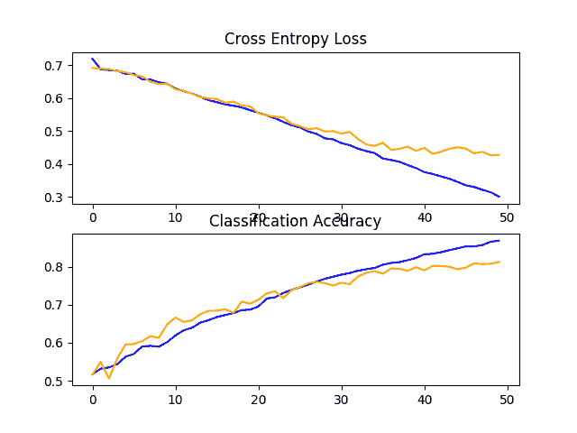
还创建了一个图形，显示了列车(蓝色)和测试(橙色)数据集上的损耗线图和另一个模型准确率图。

回顾这个图，我们可以看到模型在大约 12 个时期对训练数据集进行了过拟合。

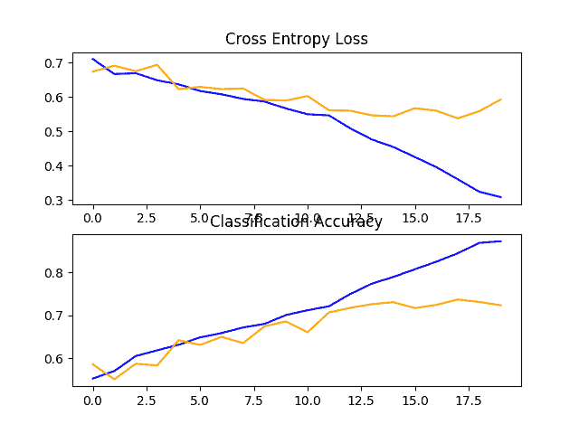
狗和猫数据集上具有一个 VGG 块的基线模型的损失和准确率学习曲线的线图

两块 VGG 模型

双块 VGG 模型扩展了一个块模型，并添加了具有 64 个过滤器的第二个块。

为了完整起见，下面提供了该模型的 define_model() 函数。

# define cnn model
def define_model():
	model = Sequential()
	model.add(Conv2D(32, (3, 3), activation='relu', kernel_initializer='he_uniform', padding='same', input_shape=(200, 200, 3)))
	model.add(MaxPooling2D((2, 2)))
	model.add(Conv2D(64, (3, 3), activation='relu', kernel_initializer='he_uniform', padding='same'))
	model.add(MaxPooling2D((2, 2)))
	model.add(Flatten())
	model.add(Dense(128, activation='relu', kernel_initializer='he_uniform'))
	model.add(Dense(1, activation='sigmoid'))
	# compile model
	opt = SGD(lr=0.001, momentum=0.9)
	model.compile(optimizer=opt, loss='binary_crossentropy', metrics=['accuracy'])
	return model

再次运行此示例将打印训练和测试数据集的大小，确认数据集加载正确。

对模型进行拟合和评估，并报告测试数据集上的表现。

Found 18697 images belonging to 2 classes.
Found 6303 images belonging to 2 classes.
> 76.646

注:考虑到算法或评估程序的随机性，或数值准确率的差异，您的结果可能会有所不同。考虑运行该示例几次，并比较平均结果。

在这种情况下，我们可以看到，该模型在表现上实现了小幅提升，从一个块的约 72%提升到两个块的约 76%

回顾学习曲线的曲线，我们可以再次看到，模型似乎过度填充了训练数据集，也许更快，在这种情况下，大约在八个训练时期。

这可能是模型容量增加的结果，我们可能预计这种更快过拟合的趋势会在下一个模型中继续。

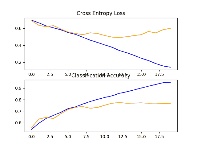
狗和猫数据集上具有两个 VGG 块的基线模型的损失和准确率学习曲线的线图

三块 VGG 模型

三块 VGG 模型扩展了两块模型，并添加了具有 128 个滤波器的第三块。

该模型的 define_model() 函数已在上一节中定义，但为了完整起见，下面再次提供。

# define cnn model
def define_model():
	model = Sequential()
	model.add(Conv2D(32, (3, 3), activation='relu', kernel_initializer='he_uniform', padding='same', input_shape=(200, 200, 3)))
	model.add(MaxPooling2D((2, 2)))
	model.add(Conv2D(64, (3, 3), activation='relu', kernel_initializer='he_uniform', padding='same'))
	model.add(MaxPooling2D((2, 2)))
	model.add(Conv2D(128, (3, 3), activation='relu', kernel_initializer='he_uniform', padding='same'))
	model.add(MaxPooling2D((2, 2)))
	model.add(Flatten())
	model.add(Dense(128, activation='relu', kernel_initializer='he_uniform'))
	model.add(Dense(1, activation='sigmoid'))
	# compile model
	opt = SGD(lr=0.001, momentum=0.9)
	model.compile(optimizer=opt, loss='binary_crossentropy', metrics=['accuracy'])
	return model

运行此示例将打印训练和测试数据集的大小，确认数据集已正确加载。

对模型进行拟合和评估，并报告测试数据集上的表现。

Found 18697 images belonging to 2 classes.
Found 6303 images belonging to 2 classes.
> 80.184

注:考虑到算法或评估程序的随机性，或数值准确率的差异，您的结果可能会有所不同。考虑运行该示例几次，并比较平均结果。

在这种情况下，我们可以看到，我们实现了表现的进一步提升，从两个模块的 76%左右提升到三个模块的 80%左右。这个结果是好的，因为它接近于该论文中使用 SVM 以大约 82%的准确度报道的现有技术水平。

回顾学习曲线的曲线，我们可以看到类似的过拟合的趋势，在这种情况下，也许可以追溯到五六世纪。

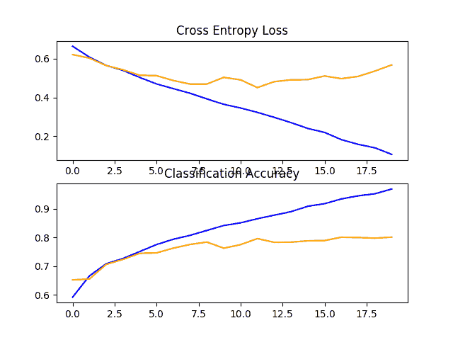
狗和猫数据集上具有三个 VGG 块的基线模型的损失和准确率学习曲线的线图

讨论

我们探索了基于 VGG 架构的三种不同模式。

结果可以总结如下，尽管我们必须假设这些结果中存在一些方差，因为算法具有随机性:

• vgg 1:72 331%
• vgg 2:76 646%
• VGG 3 : 80，184%

随着容量的增加，我们看到了表现提高的趋势，但在运行中也出现了越来越早的过拟合的类似情况。

结果表明，该模型将可能受益于正则化技术。这可能包括技术，如丢弃，权重下降，和数据增加。后者还可以通过扩展训练数据集来鼓励模型学习位置不变的特征，从而提高表现。

开发模型改进

在上一节中，我们使用 VGG 风格的模块开发了一个基线模型，并发现了随着模型容量的增加而提高表现的趋势。

在本节中，我们将从具有三个 VGG 区块(即 VGG 3)的基线模型开始，并探索模型的一些简单改进。

从训练期间查看模型的学习曲线来看，模型显示出强烈的过拟合迹象。我们可以探索两种方法来尝试解决这种过拟合的问题:丢弃正规化和数据增加。

这两种方法都有望减缓训练过程中的改进速度，并有望对抗训练数据集的过拟合。因此，我们将训练阶段的数量从 20 个增加到 50 个，以给模型更多的细化空间。

丢弃正规化

脱落正则化是一种计算量小的正则化深度神经网络的方法。

丢弃的工作原理是从概率上移除，或者“T0”从“T1”中移除，输入到一个层，该层可以是数据样本中的输入变量或者来自前一层的激活。它具有模拟大量具有非常不同的网络结构的网络的效果，并且反过来使得网络中的节点通常对输入更加鲁棒。

有关丢弃的更多信息，请参阅帖子:

• 如何利用 Keras 中的丢弃正则化减少过拟合

通常，每个 VGG 模块后可以施加少量压降，更多压降施加于模型输出层附近的全连接层。

下面是添加了 Dropout 的基线模型的更新版本的 define_model() 函数。在这种情况下，在每个 VGG 块之后应用 20%的丢失率，在模型的分类器部分的完全连接层之后应用更大的 50%的丢失率。

# define cnn model
def define_model():
	model = Sequential()
	model.add(Conv2D(32, (3, 3), activation='relu', kernel_initializer='he_uniform', padding='same', input_shape=(200, 200, 3)))
	model.add(MaxPooling2D((2, 2)))
	model.add(Dropout(0.2))
	model.add(Conv2D(64, (3, 3), activation='relu', kernel_initializer='he_uniform', padding='same'))
	model.add(MaxPooling2D((2, 2)))
	model.add(Dropout(0.2))
	model.add(Conv2D(128, (3, 3), activation='relu', kernel_initializer='he_uniform', padding='same'))
	model.add(MaxPooling2D((2, 2)))
	model.add(Dropout(0.2))
	model.add(Flatten())
	model.add(Dense(128, activation='relu', kernel_initializer='he_uniform'))
	model.add(Dropout(0.5))
	model.add(Dense(1, activation='sigmoid'))
	# compile model
	opt = SGD(lr=0.001, momentum=0.9)
	model.compile(optimizer=opt, loss='binary_crossentropy', metrics=['accuracy'])
	return model

为了完整起见，下面列出了基线模型的完整代码列表，并在犬猫数据集上增加了 drop。

# baseline model with dropout for the dogs vs cats dataset
import sys
from matplotlib import pyplot
from keras.utils import to_categorical
from keras.models import Sequential
from keras.layers import Conv2D
from keras.layers import MaxPooling2D
from keras.layers import Dense
from keras.layers import Flatten
from keras.layers import Dropout
from keras.optimizers import SGD
from keras.preprocessing.image import ImageDataGenerator

# define cnn model
def define_model():
	model = Sequential()
	model.add(Conv2D(32, (3, 3), activation='relu', kernel_initializer='he_uniform', padding='same', input_shape=(200, 200, 3)))
	model.add(MaxPooling2D((2, 2)))
	model.add(Dropout(0.2))
	model.add(Conv2D(64, (3, 3), activation='relu', kernel_initializer='he_uniform', padding='same'))
	model.add(MaxPooling2D((2, 2)))
	model.add(Dropout(0.2))
	model.add(Conv2D(128, (3, 3), activation='relu', kernel_initializer='he_uniform', padding='same'))
	model.add(MaxPooling2D((2, 2)))
	model.add(Dropout(0.2))
	model.add(Flatten())
	model.add(Dense(128, activation='relu', kernel_initializer='he_uniform'))
	model.add(Dropout(0.5))
	model.add(Dense(1, activation='sigmoid'))
	# compile model
	opt = SGD(lr=0.001, momentum=0.9)
	model.compile(optimizer=opt, loss='binary_crossentropy', metrics=['accuracy'])
	return model

# plot diagnostic learning curves
def summarize_diagnostics(history):
	# plot loss
	pyplot.subplot(211)
	pyplot.title('Cross Entropy Loss')
	pyplot.plot(history.history['loss'], color='blue', label='train')
	pyplot.plot(history.history['val_loss'], color='orange', label='test')
	# plot accuracy
	pyplot.subplot(212)
	pyplot.title('Classification Accuracy')
	pyplot.plot(history.history['accuracy'], color='blue', label='train')
	pyplot.plot(history.history['val_accuracy'], color='orange', label='test')
	# save plot to file
	filename = sys.argv[0].split('/')[-1]
	pyplot.savefig(filename + '_plot.png')
	pyplot.close()

# run the test harness for evaluating a model
def run_test_harness():
	# define model
	model = define_model()
	# create data generator
	datagen = ImageDataGenerator(rescale=1.0/255.0)
	# prepare iterator
	train_it = datagen.flow_from_directory('dataset_dogs_vs_cats/train/',
		class_mode='binary', batch_size=64, target_size=(200, 200))
	test_it = datagen.flow_from_directory('dataset_dogs_vs_cats/test/',
		class_mode='binary', batch_size=64, target_size=(200, 200))
	# fit model
	history = model.fit_generator(train_it, steps_per_epoch=len(train_it),
		validation_data=test_it, validation_steps=len(test_it), epochs=50, verbose=0)
	# evaluate model
	_, acc = model.evaluate_generator(test_it, steps=len(test_it), verbose=0)
	print('> %.3f' % (acc * 100.0))
	# learning curves
	summarize_diagnostics(history)

# entry point, run the test harness
run_test_harness()

运行该示例首先适合模型，然后在等待测试数据集上报告模型表现。

注:考虑到算法或评估程序的随机性，或数值准确率的差异，您的结果可能会有所不同。考虑运行该示例几次，并比较平均结果。

在这种情况下，我们可以看到模型表现的小幅提升，从基线模型的 80%左右的准确率提升到增加了脱落的 81%左右。

Found 18697 images belonging to 2 classes.
Found 6303 images belonging to 2 classes.
> 81.279

回顾学习曲线，我们可以看到丢弃对模型在训练集和测试集上的改进速度都有影响。

过拟合已经减少或延迟，尽管表现可能在接近运行结束时开始停滞。

结果表明，进一步的训练阶段可能导致模型的进一步改进。除了训练时期的增加之外，探索 VGG 街区之后稍高的丢弃率也可能是有趣的。

犬猫数据集上缺失基线模型的损失和准确率学习曲线的线图

图像数据增长

图像数据扩充是一种技术，可用于通过在数据集中创建图像的修改版本来人工扩展训练数据集的大小。

在更多的数据上训练深度学习神经网络模型可以产生更熟练的模型，并且增强技术可以创建图像的变化，这可以提高拟合模型将他们所学知识推广到新图像的能力。

数据扩充也可以作为一种正则化技术，向训练数据添加噪声，并鼓励模型学习相同的特征，这些特征在输入中的位置是不变的。

对狗和猫的输入照片进行一些小的改变可能对这个问题有用，比如小的移动和水平翻转。这些扩充可以被指定为用于训练数据集的 ImageDataGenerator 的参数。增强不应用于测试数据集，因为我们希望在未修改的照片上评估模型的表现。

这要求我们为训练和测试数据集有一个单独的 ImageDataGenerator 实例，然后为从各自的数据生成器创建的训练和测试集有迭代器。例如:

# create data generators
train_datagen = ImageDataGenerator(rescale=1.0/255.0,
	width_shift_range=0.1, height_shift_range=0.1, horizontal_flip=True)
test_datagen = ImageDataGenerator(rescale=1.0/255.0)
# prepare iterators
train_it = train_datagen.flow_from_directory('dataset_dogs_vs_cats/train/',
	class_mode='binary', batch_size=64, target_size=(200, 200))
test_it = test_datagen.flow_from_directory('dataset_dogs_vs_cats/test/',
	class_mode='binary', batch_size=64, target_size=(200, 200))

在这种情况下，训练数据集中的照片将通过小的(10%)随机水平和垂直移动以及创建照片镜像的随机水平翻转进行增强。训练和测试步骤中的照片将以相同的方式缩放其像素值。

为了完整起见，下面列出了带有狗和猫数据集训练数据扩充的基线模型的完整代码列表。

# baseline model with data augmentation for the dogs vs cats dataset
import sys
from matplotlib import pyplot
from keras.utils import to_categorical
from keras.models import Sequential
from keras.layers import Conv2D
from keras.layers import MaxPooling2D
from keras.layers import Dense
from keras.layers import Flatten
from keras.optimizers import SGD
from keras.preprocessing.image import ImageDataGenerator

# define cnn model
def define_model():
	model = Sequential()
	model.add(Conv2D(32, (3, 3), activation='relu', kernel_initializer='he_uniform', padding='same', input_shape=(200, 200, 3)))
	model.add(MaxPooling2D((2, 2)))
	model.add(Conv2D(64, (3, 3), activation='relu', kernel_initializer='he_uniform', padding='same'))
	model.add(MaxPooling2D((2, 2)))
	model.add(Conv2D(128, (3, 3), activation='relu', kernel_initializer='he_uniform', padding='same'))
	model.add(MaxPooling2D((2, 2)))
	model.add(Flatten())
	model.add(Dense(128, activation='relu', kernel_initializer='he_uniform'))
	model.add(Dense(1, activation='sigmoid'))
	# compile model
	opt = SGD(lr=0.001, momentum=0.9)
	model.compile(optimizer=opt, loss='binary_crossentropy', metrics=['accuracy'])
	return model

# plot diagnostic learning curves
def summarize_diagnostics(history):
	# plot loss
	pyplot.subplot(211)
	pyplot.title('Cross Entropy Loss')
	pyplot.plot(history.history['loss'], color='blue', label='train')
	pyplot.plot(history.history['val_loss'], color='orange', label='test')
	# plot accuracy
	pyplot.subplot(212)
	pyplot.title('Classification Accuracy')
	pyplot.plot(history.history['accuracy'], color='blue', label='train')
	pyplot.plot(history.history['val_accuracy'], color='orange', label='test')
	# save plot to file
	filename = sys.argv[0].split('/')[-1]
	pyplot.savefig(filename + '_plot.png')
	pyplot.close()

# run the test harness for evaluating a model
def run_test_harness():
	# define model
	model = define_model()
	# create data generators
	train_datagen = ImageDataGenerator(rescale=1.0/255.0,
		width_shift_range=0.1, height_shift_range=0.1, horizontal_flip=True)
	test_datagen = ImageDataGenerator(rescale=1.0/255.0)
	# prepare iterators
	train_it = train_datagen.flow_from_directory('dataset_dogs_vs_cats/train/',
		class_mode='binary', batch_size=64, target_size=(200, 200))
	test_it = test_datagen.flow_from_directory('dataset_dogs_vs_cats/test/',
		class_mode='binary', batch_size=64, target_size=(200, 200))
	# fit model
	history = model.fit_generator(train_it, steps_per_epoch=len(train_it),
		validation_data=test_it, validation_steps=len(test_it), epochs=50, verbose=0)
	# evaluate model
	_, acc = model.evaluate_generator(test_it, steps=len(test_it), verbose=0)
	print('> %.3f' % (acc * 100.0))
	# learning curves
	summarize_diagnostics(history)

# entry point, run the test harness
run_test_harness()

运行该示例首先适合模型，然后在等待测试数据集上报告模型表现。

注:考虑到算法或评估程序的随机性，或数值准确率的差异，您的结果可能会有所不同。考虑运行该示例几次，并比较平均结果。

在这种情况下，我们可以看到表现提升了大约 5%，从基线模型的大约 80%提升到具有简单数据增加的基线模型的大约 85%。

> 85.816

回顾学习曲线，我们可以看到该模型似乎能够进一步学习，即使在运行结束时，训练和测试数据集上的损失仍在减少。用 100 个或更多的时代重复这个实验很可能会产生一个表现更好的模型。

探索可以进一步鼓励学习不随其在输入中的位置而变化的特征的其他扩展可能是有趣的，例如微小的旋转和缩放。

狗和猫数据集上具有数据增加的基线模型的损失和准确率学习曲线的线图

讨论

我们对基线模型进行了三种不同的改进。

结果可以总结如下，尽管我们必须假设这些结果中存在一些方差，因为算法具有随机性:

• 基线 VGG3 +丢弃率:81.279%
• 基线 VGG3 +数据增加:85 816

正如所怀疑的那样，正则化技术的加入减缓了学习算法的进程，减少了过拟合，从而提高了保持数据集的表现。这两种方法的结合以及训练时期数量的进一步增加很可能会导致进一步的改进。

这只是可以在这个数据集上探索的改进类型的开始。除了对所描述的正则化方法进行调整之外，还可以探索其他正则化方法，例如权重衰减和提前停止。

可能值得探索学习算法的变化，例如学习率的变化，学习率时间表的使用，或者自适应学习率，例如亚当。

替代模型架构也值得探索。所选的基准模型预计会提供比解决此问题所需的更多的容量，较小的模型可能会更快地进行训练，从而提高表现。

探索迁移学习

迁移学习涉及使用在相关任务上训练的模型的全部或部分。

Keras 提供了一系列预先训练好的模型，可以通过 Keras 应用 API 全部或部分加载和使用。

迁移学习的一个有用模型是 VGG 模型之一，例如 VGG-16，它有 16 层，在开发时，在 ImageNet 照片分类挑战中取得了顶级表现。

该模型由两个主要部分组成，模型的特征提取器部分由 VGG 块组成，模型的分类器部分由完全连接的层和输出层组成。

我们可以使用模型的特征提取部分，并添加一个新的分类器部分的模型，这是量身定制的狗和猫数据集。具体来说，我们可以在训练过程中保持所有卷积层的权重固定，只训练新的完全连接的层，这些层将学习解释从模型中提取的特征并进行二进制分类。

这可以通过加载 VGG-16 模型，从模型的输出端移除全连接层，然后添加新的全连接层来解释模型输出并进行预测来实现。通过将“ include_top ”参数设置为“ False ，可以自动移除模型的分类器部分，这也要求为模型指定输入的形状，在本例中为(224，224，3)。这意味着加载的模型在最后一个最大池层结束，之后我们可以手动添加一个扁平化层和新的 clasifier 层。

下面的 define_model() 函数实现了这一点，并返回一个准备训练的新模型。

# define cnn model
def define_model():
	# load model
	model = VGG16(include_top=False, input_shape=(224, 224, 3))
	# mark loaded layers as not trainable
	for layer in model.layers:
		layer.trainable = False
	# add new classifier layers
	flat1 = Flatten()(model.layers[-1].output)
	class1 = Dense(128, activation='relu', kernel_initializer='he_uniform')(flat1)
	output = Dense(1, activation='sigmoid')(class1)
	# define new model
	model = Model(inputs=model.inputs, outputs=output)
	# compile model
	opt = SGD(lr=0.001, momentum=0.9)
	model.compile(optimizer=opt, loss='binary_crossentropy', metrics=['accuracy'])
	return model

一旦创建，我们就可以像以前一样在训练数据集上训练模型。

在这种情况下，不需要大量的训练，因为只有新的完全连接和输出层具有可训练的权重。因此，我们将把训练时期的数量固定在 10 个。

VGG16 模型在特定的 ImageNet 挑战数据集上进行了训练。因此，它被配置为期望输入图像具有 224×224 像素的形状。当从狗和猫的数据集中加载照片时，我们将使用这个作为目标大小。

该模型还希望图像居中。也就是说，从输入中减去在 ImageNet 训练数据集上计算的每个通道(红色、绿色和蓝色)的平均像素值。Keras 通过*预处理 _ 输入()*功能提供了一个为单个照片执行该准备的功能。然而，我们可以通过将“ featurewise_center ”参数设置为“ True ”并手动指定居中时使用的平均像素值作为来自 ImageNet 训练数据集的平均值来达到相同的效果:[123.68，116.779，103.939]。

下面列出了狗和猫数据集上用于迁移学习的 VGG 模型的完整代码列表。

# vgg16 model used for transfer learning on the dogs and cats dataset
import sys
from matplotlib import pyplot
from keras.utils import to_categorical
from keras.applications.vgg16 import VGG16
from keras.models import Model
from keras.layers import Dense
from keras.layers import Flatten
from keras.optimizers import SGD
from keras.preprocessing.image import ImageDataGenerator

# define cnn model
def define_model():
	# load model
	model = VGG16(include_top=False, input_shape=(224, 224, 3))
	# mark loaded layers as not trainable
	for layer in model.layers:
		layer.trainable = False
	# add new classifier layers
	flat1 = Flatten()(model.layers[-1].output)
	class1 = Dense(128, activation='relu', kernel_initializer='he_uniform')(flat1)
	output = Dense(1, activation='sigmoid')(class1)
	# define new model
	model = Model(inputs=model.inputs, outputs=output)
	# compile model
	opt = SGD(lr=0.001, momentum=0.9)
	model.compile(optimizer=opt, loss='binary_crossentropy', metrics=['accuracy'])
	return model

# plot diagnostic learning curves
def summarize_diagnostics(history):
	# plot loss
	pyplot.subplot(211)
	pyplot.title('Cross Entropy Loss')
	pyplot.plot(history.history['loss'], color='blue', label='train')
	pyplot.plot(history.history['val_loss'], color='orange', label='test')
	# plot accuracy
	pyplot.subplot(212)
	pyplot.title('Classification Accuracy')
	pyplot.plot(history.history['accuracy'], color='blue', label='train')
	pyplot.plot(history.history['val_accuracy'], color='orange', label='test')
	# save plot to file
	filename = sys.argv[0].split('/')[-1]
	pyplot.savefig(filename + '_plot.png')
	pyplot.close()

# run the test harness for evaluating a model
def run_test_harness():
	# define model
	model = define_model()
	# create data generator
	datagen = ImageDataGenerator(featurewise_center=True)
	# specify imagenet mean values for centering
	datagen.mean = [123.68, 116.779, 103.939]
	# prepare iterator
	train_it = datagen.flow_from_directory('dataset_dogs_vs_cats/train/',
		class_mode='binary', batch_size=64, target_size=(224, 224))
	test_it = datagen.flow_from_directory('dataset_dogs_vs_cats/test/',
		class_mode='binary', batch_size=64, target_size=(224, 224))
	# fit model
	history = model.fit_generator(train_it, steps_per_epoch=len(train_it),
		validation_data=test_it, validation_steps=len(test_it), epochs=10, verbose=1)
	# evaluate model
	_, acc = model.evaluate_generator(test_it, steps=len(test_it), verbose=0)
	print('> %.3f' % (acc * 100.0))
	# learning curves
	summarize_diagnostics(history)

# entry point, run the test harness
run_test_harness()

运行该示例首先适合模型，然后在等待测试数据集上报告模型表现。

注:考虑到算法或评估程序的随机性，或数值准确率的差异，您的结果可能会有所不同。考虑运行该示例几次，并比较平均结果。

在这种情况下，我们可以看到该模型在保持测试数据集上以大约 97%的分类准确率获得了非常令人印象深刻的结果。

Found 18697 images belonging to 2 classes.
Found 6303 images belonging to 2 classes.
> 97.636

回顾学习曲线，我们可以看到模型很快拟合数据集。它没有表现出很强的过拟合，尽管结果表明，也许分类器的额外容量和/或正则化的使用可能是有帮助的。

对这种方法可以进行许多改进，包括向模型的分类器部分添加缺失正则化，甚至可能微调模型的特征检测器部分中的一些或所有层的权重。

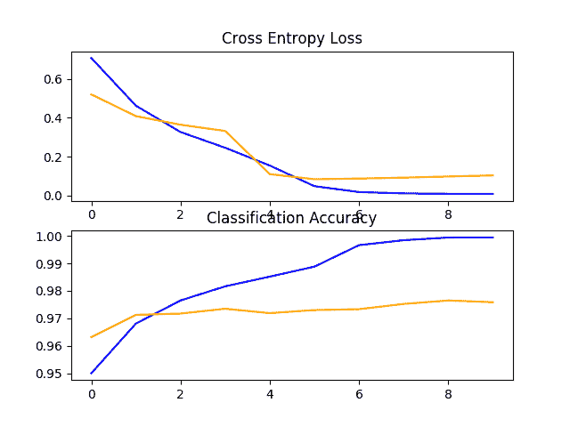
狗和猫数据集上 VGG16 迁移学习模型的损失和准确率学习曲线的线图

如何最终确定模型并做出预测

只要我们有想法，有时间和资源来测试，模型改进的过程可能会持续很长时间。

在某些时候，必须选择并采用最终的模型配置。在这种情况下，我们将保持事情简单，并使用 VGG-16 转移学习方法作为最终模型。

首先，我们将通过在整个训练数据集上拟合模型并将模型保存到文件中以备后用来最终确定我们的模型。然后，我们将加载保存的模型，并使用它对单个图像进行预测。

准备最终数据集

最终模型通常适合所有可用数据，例如所有训练和测试数据集的组合。

在本教程中，我们将仅在训练数据集上演示最终模型拟合，因为我们只有训练数据集的标签。

第一步是准备训练数据集，以便通过 flow_from_directory() 函数由 ImageDataGenerator 类加载。具体来说，我们需要创建一个新的目录，将所有训练图像组织到狗/ 和猫/ 子目录中，而不将其分离到训练/ 或测试/ 目录中。

这可以通过更新我们在教程开始时开发的脚本来实现。在这种情况下，我们将为整个训练数据集创建一个新的*finalize _ dogs _ vs _ cat/文件夹，其中包含 dogs/ 和cat/*子文件夹。

结构如下所示:

finalize_dogs_vs_cats
├── cats
└── dogs

为了完整起见，下面列出了更新后的脚本。

# organize dataset into a useful structure
from os import makedirs
from os import listdir
from shutil import copyfile
# create directories
dataset_home = 'finalize_dogs_vs_cats/'
# create label subdirectories
labeldirs = ['dogs/', 'cats/']
for labldir in labeldirs:
	newdir = dataset_home + labldir
	makedirs(newdir, exist_ok=True)
# copy training dataset images into subdirectories
src_directory = 'dogs-vs-cats/train/'
for file in listdir(src_directory):
	src = src_directory + '/' + file
	if file.startswith('cat'):
		dst = dataset_home + 'cats/'  + file
		copyfile(src, dst)
	elif file.startswith('dog'):
		dst = dataset_home + 'dogs/'  + file
		copyfile(src, dst)

保存最终模型

我们现在准备在整个训练数据集上拟合最终模型。

必须更新 flow_from_directory() 以加载新的*finalize _ dogs _ vs _ cat/*目录中的所有图像。

# prepare iterator
train_it = datagen.flow_from_directory('finalize_dogs_vs_cats/',
	class_mode='binary', batch_size=64, target_size=(224, 224))

此外，对 fit_generator() 的调用不再需要指定验证数据集。

# fit model
model.fit_generator(train_it, steps_per_epoch=len(train_it), epochs=10, verbose=0)

一旦合适，我们可以通过调用模型上的 save() 函数将最终模型保存到一个 H5 文件中，并传入选择的文件名。

# save model
model.save('final_model.h5')

注意，保存和加载 Keras 模型需要在您的工作站上安装 h5py 库。

下面列出了在训练数据集上拟合最终模型并将其保存到文件中的完整示例。

# save the final model to file
from keras.applications.vgg16 import VGG16
from keras.models import Model
from keras.layers import Dense
from keras.layers import Flatten
from keras.optimizers import SGD
from keras.preprocessing.image import ImageDataGenerator

# define cnn model
def define_model():
	# load model
	model = VGG16(include_top=False, input_shape=(224, 224, 3))
	# mark loaded layers as not trainable
	for layer in model.layers:
		layer.trainable = False
	# add new classifier layers
	flat1 = Flatten()(model.layers[-1].output)
	class1 = Dense(128, activation='relu', kernel_initializer='he_uniform')(flat1)
	output = Dense(1, activation='sigmoid')(class1)
	# define new model
	model = Model(inputs=model.inputs, outputs=output)
	# compile model
	opt = SGD(lr=0.001, momentum=0.9)
	model.compile(optimizer=opt, loss='binary_crossentropy', metrics=['accuracy'])
	return model

# run the test harness for evaluating a model
def run_test_harness():
# define model
	model = define_model()
	# create data generator
	datagen = ImageDataGenerator(featurewise_center=True)
	# specify imagenet mean values for centering
	datagen.mean = [123.68, 116.779, 103.939]
	# prepare iterator
	train_it = datagen.flow_from_directory('finalize_dogs_vs_cats/',
		class_mode='binary', batch_size=64, target_size=(224, 224))
	# fit model
	model.fit_generator(train_it, steps_per_epoch=len(train_it), epochs=10, verbose=0)
	# save model
	model.save('final_model.h5')

# entry point, run the test harness
run_test_harness()

运行此示例后，您将在当前工作目录中拥有一个名为“ final_model.h5 ”的 81 兆字节大文件。

作出预测

我们可以使用保存的模型对新图像进行预测。

该模型假设新图像是彩色的，并且它们已经被分割，因此一幅图像至少包含一只狗或猫。

下面是从狗和猫比赛的测试数据集中提取的图像。它没有标签，但我们可以清楚地看出它是一张狗的照片。您可以将其保存在当前工作目录中，文件名为“ sample_image.jpg ”。

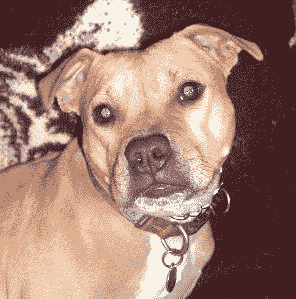
Dog (sample_image.jpg)

• 下载狗狗照片(sample_image.jpg)

我们将假装这是一个全新的、看不见的图像，按照要求的方式准备，看看我们如何使用保存的模型来预测图像所代表的整数。对于这个例子，我们期望类“ 1 ”为“狗”。

注意:图像的子目录，每个类一个，由 flow_from_directory() 函数按字母顺序加载，并为每个类分配一个整数。子目录“猫”在“狗之前，因此类标签被分配了整数:猫=0，狗=1 。这可以通过训练模型时调用 flow_from_directory() 中的“类参数来更改。

首先，我们可以加载图像，并强制其大小为 224×224 像素。然后可以调整加载图像的大小，使其在数据集中具有单个样本。像素值也必须居中，以匹配模型训练期间准备数据的方式。 load_image() 函数实现了这一点，并将返回已加载的准备分类的图像。

# load and prepare the image
def load_image(filename):
	# load the image
	img = load_img(filename, target_size=(224, 224))
	# convert to array
	img = img_to_array(img)
	# reshape into a single sample with 3 channels
	img = img.reshape(1, 224, 224, 3)
	# center pixel data
	img = img.astype('float32')
	img = img - [123.68, 116.779, 103.939]
	return img

接下来，我们可以像上一节一样加载模型，并调用 predict()函数将图像中的内容预测为“ 0 ”和“ 1 之间的数字，分别表示“猫”和“狗”。

# predict the class
result = model.predict(img)

下面列出了完整的示例。

# make a prediction for a new image.
from keras.preprocessing.image import load_img
from keras.preprocessing.image import img_to_array
from keras.models import load_model

# load and prepare the image
def load_image(filename):
	# load the image
	img = load_img(filename, target_size=(224, 224))
	# convert to array
	img = img_to_array(img)
	# reshape into a single sample with 3 channels
	img = img.reshape(1, 224, 224, 3)
	# center pixel data
	img = img.astype('float32')
	img = img - [123.68, 116.779, 103.939]
	return img

# load an image and predict the class
def run_example():
	# load the image
	img = load_image('sample_image.jpg')
	# load model
	model = load_model('final_model.h5')
	# predict the class
	result = model.predict(img)
	print(result[0])

# entry point, run the example
run_example()

运行该示例首先加载和准备图像，加载模型，然后正确预测加载的图像代表“狗或类“ 1 ”。

1

扩展ˌ扩张

本节列出了一些您可能希望探索的扩展教程的想法。

• 调整正则化。探索基线模型中使用的正则化技术的微小变化，例如不同的丢弃率和不同的图像扩充。
• 调整学习率。探索对用于训练基线模型的学习算法的更改，例如替代学习率、学习率计划或自适应学习率算法，例如 Adam。
• 交替预训练模型。探索一种替代的预先训练的模型，用于问题的迁移学习，如 Inception 或 ResNet。

如果你探索这些扩展，我很想知道。
在下面的评论中发表你的发现。

进一步阅读

如果您想更深入地了解这个主题，本节将提供更多资源。

报纸

• Asirra:利用兴趣对齐的手动图像分类的验证码，2007。
• 机器学习攻击阿西拉验证码，2007。
• overheat:使用卷积网络的集成识别、定位和检测，2013。

应用程序接口

• Keras 应用程序接口
• Keras 图像处理 API
• Keras 顺序模型 API

文章

• 狗 vs 猫卡格尔比赛。
• 狗 vs 猫 Redux:内核版。
• 狗 vs 猫数据集，卡格尔。
• 用很少的数据构建强大的图像分类模型，2016。

摘要

在本教程中，您发现了如何开发卷积神经网络来对狗和猫的照片进行分类。

具体来说，您了解到:

• 如何加载和准备狗和猫的照片进行建模？
• 如何从零开始开发卷积神经网络进行照片分类并提高模型表现？
• 如何利用迁移学习开发照片分类模型？

你有什么问题吗？
在下面的评论中提问，我会尽力回答。

亚马逊雨林卫星照片多标签分类

原文：https://machinelearningmastery.com/how-to-develop-a-convolutional-neural-network-to-classify-satellite-photos-of-the-amazon-rainforest/

最后更新于 2020 年 8 月 24 日

行星数据集已经成为一个标准的计算机视觉基准，它涉及对亚马逊热带雨林卫星照片的内容进行多标签分类或标记。

该数据集是 Kaggle 网站上数据科学竞赛的基础，并得到了有效解决。然而，它可以作为学习和实践如何从零开始开发、评估和使用卷积深度学习神经网络进行图像分类的基础。

这包括如何开发一个健壮的测试工具来评估模型的表现，如何探索模型的改进，以及如何保存模型并在以后加载它来对新数据进行预测。

在本教程中，您将发现如何开发卷积神经网络来对亚马逊热带雨林的卫星照片进行分类。

完成本教程后，您将知道:

• 如何加载准备亚马逊热带雨林卫星照片进行建模？
• 如何从零开始开发卷积神经网络进行照片分类并提高模型表现？
• 如何开发最终模型，并使用它对新数据进行特别预测。

用我的新书计算机视觉深度学习启动你的项目，包括分步教程和所有示例的 Python 源代码文件。

我们开始吧。

• 更新 2019 年 9 月:更新了如何下载数据集的说明。
• 2019 年 10 月更新:针对 Keras 2.3.0 和 TensorFlow 2.0.0 更新。

如何开发卷积神经网络来对亚马逊雨林的卫星照片进行分类安娜&米歇尔的照片，保留部分权利。

教程概述

本教程分为七个部分；它们是:

1. 行星数据集简介
2. 如何为建模准备数据
3. 模型评估方法
4. 如何评估基线模型
5. 如何提高模型表现
6. 如何使用迁移学习
7. 如何最终确定模型并做出预测

行星数据集简介

“T0”星球:从太空了解亚马逊比赛于 2017 年在卡格尔举行。

比赛涉及将从巴西亚马逊雨林太空拍摄的卫星图像小方块按照“农业”、“T2】晴空、“T4】水等 17 类进行分类。鉴于竞赛的名称，数据集通常简称为“行星数据集”。

*彩色图像以 256×256 像素的 TIFF 和 JPEG 格式提供。训练数据集中总共提供了 40，779 幅图像，测试集中提供了 40，669 幅需要预测的图像。

该问题是一个多标签图像分类任务的例子，其中必须为每个标签预测一个或多个类别标签。这不同于多类别分类，在多类别分类中，每个图像被分配多个类别中的一个。

为训练数据集中的每个图像提供了多个类别标签，并附带了一个将图像文件名映射到字符串类别标签的文件。

比赛进行了大约四个月(2017 年 4 月至 7 月)，共有 938 个团队参加，围绕数据准备、数据扩充和卷积神经网络的使用展开了大量讨论。

比赛由名为“ bestfitting ”的竞争对手赢得，在 66%的测试数据集上，公共排行榜 F-beta 评分为 0.93398，在 34%的测试数据集上，私有排行榜 F-beta 评分为 0.93317。他的方法在帖子“星球:从太空理解亚马逊，第一名得主的采访”中有所描述，并涉及大量模型的流水线和集成，其中大部分是具有转移学习的卷积神经网络。

这是一场具有挑战性的比赛，尽管数据集仍然是免费提供的(如果你有一个 Kaggle 帐户)，并为使用卷积神经网络对航空和卫星数据集进行图像分类提供了一个很好的基准问题。

因此，在这项任务中，使用手动设计的卷积神经网络获得大于 80 的 F-β分数和使用转移学习获得 89+的 F-β分数是常规。

如何为建模准备数据

第一步是下载数据集。

为了下载数据文件，您必须有一个 Kaggle 帐户。如果你没有卡格尔账号，可以在这里创建一个:卡格尔主页。

数据集可以从行星数据页面下载。此页面列出了为比赛提供的所有文件，尽管我们不需要下载所有文件。

• 星球:从太空数据下载页面了解亚马逊

下载数据集前，必须点击加入竞赛按钮。您可能需要同意竞赛规则，然后数据集将可供下载。

加入竞争

要下载给定的文件，当你用鼠标悬停在文件上时，点击出现在文件旁边的下载按钮的小图标(在右侧)，如下图所示。

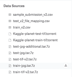
下载行星数据集文件的下载按钮示例

本教程所需的具体文件如下:

• 列车-jpg.tar.7z (600MB)
• train_v2.csv.zip (159KB)

**注意:**JPEG zip 文件可能没有. 7z 扩展名。如果是，请下载。焦油版本。

下载数据集文件后，必须将其解压缩。那个。CSV 文件的 zip 文件可以使用您最喜欢的解压程序解压。

那个。 7z 包含 JPEG 图像的文件也可以使用您最喜欢的解压缩程序解压缩。如果这是一种新的 zip 格式，您可能需要额外的软件，例如 MacOS 上的“Unarchiver”软件，或者许多平台上的 p7zip 。

例如，在大多数基于 POSIX 的工作站的命令行上，可以使用 p7zip 和 tar 文件对. 7z 文件进行解压缩，如下所示:

7z x test-jpg.tar.7z
tar -xvf test-jpg.tar
7z x train-jpg.tar.7z
tar -xvf train-jpg.tar

解压缩后，您将拥有一个 CSV 文件和一个位于当前工作目录中的目录，如下所示:

train-jpg/
train_v2.csv

检查文件夹，你会看到许多 jpeg 文件。

检查 train_v2.csv 文件，您将看到训练数据集中的 jpeg 文件的映射( train-jpg/ )以及它们到类标签的映射，每个类标签用空格分隔；例如:

image_name,tags
train_0,haze primary
train_1,agriculture clear primary water
train_2,clear primary
train_3,clear primary
train_4,agriculture clear habitation primary road
...

建模前必须准备好数据集。

我们至少有两种方法可以探索；它们是:内存方法和渐进加载方法。

准备数据集的目的是在拟合模型时将整个训练数据集加载到内存中。这将需要一台具有足够内存来保存所有图像的机器(例如 32GB 或 64GB 的内存)，例如亚马逊 EC2 实例，尽管训练模型会快得多。

或者，数据集可以在训练期间根据需要逐批加载。这需要开发一个数据生成器。训练模型会慢得多，但训练可以在内存较少的工作站上进行(例如 8GB 或 16GB)。

在本教程中，我们将使用前一种方法。因此，我强烈建议您在具有足够内存和 GPU 访问权限的亚马逊 EC2 实例上运行本教程，例如价格合理的深度学习 AMI(亚马逊 Linux) AMI 上的 p3.2xlarge 实例，每小时费用约为 3 美元。有关如何为深度学习设置亚马逊 EC2 实例的分步教程，请参见文章:

• 如何设置亚马逊 AWS EC2 GPUs 训练深度学习模型(分步)

如果使用 EC2 实例不是您的选择，那么我将在下面给出提示，说明如何进一步减小训练数据集的大小，使其适合您工作站上的内存，以便您可以完成本教程。

可视化数据集

第一步是检查训练数据集中的一些图像。

我们可以通过加载一些图像并使用 Matplotlib 在一个图形中绘制多个图像来实现这一点。

下面列出了完整的示例。

# plot the first 9 images in the planet dataset
from matplotlib import pyplot
from matplotlib.image import imread
# define location of dataset
folder = 'train-jpg/'
# plot first few images
for i in range(9):
	# define subplot
	pyplot.subplot(330 + 1 + i)
	# define filename
	filename = folder + 'train_' + str(i) + '.jpg'
	# load image pixels
	image = imread(filename)
	# plot raw pixel data
	pyplot.imshow(image)
# show the figure
pyplot.show()

运行该示例会创建一个图形，绘制训练数据集中的前九幅图像。

我们可以看到这些图像确实是雨林的卫星照片。一些显示明显的雾霾，另一些显示树木、道路或河流和其他结构。

这些图表明，建模可能会受益于数据扩充以及简单的技术，使图像中的特征更加明显。

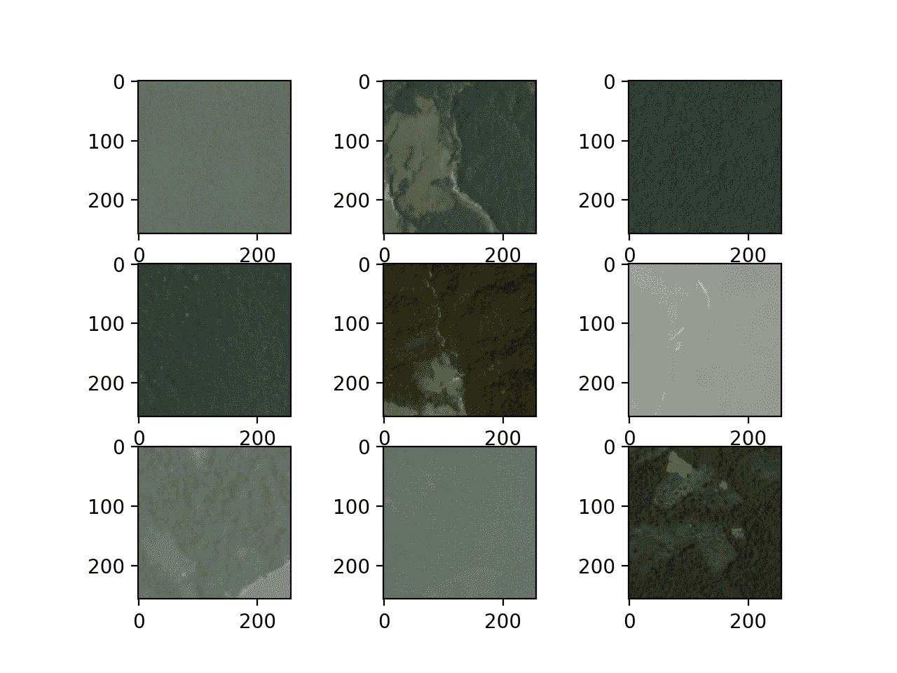
图中显示了行星数据集中的前九幅图像

创建映射

下一步包括理解可以分配给每个图像的标签。

我们可以直接使用 read_csv()熊猫函数加载训练数据集( train_v2.csv )的 CSV 映射文件。

下面列出了完整的示例。

# load and summarize the mapping file for the planet dataset
from pandas import read_csv
# load file as CSV
filename = 'train_v2.csv'
mapping_csv = read_csv(filename)
# summarize properties
print(mapping_csv.shape)
print(mapping_csv[:10])

运行该示例首先总结训练数据集的形状。我们可以看到，映射文件确实有 40，479 个已知的训练图像。

接下来，总结文件的前 10 行。我们可以看到，文件的第二列包含一个用空格分隔的标签列表，用于分配给每个图像。

(40479, 2)

  image_name                                         tags
0    train_0                                 haze primary
1    train_1              agriculture clear primary water
2    train_2                                clear primary
3    train_3                                clear primary
4    train_4    agriculture clear habitation primary road
5    train_5                           haze primary water
6    train_6  agriculture clear cultivation primary water
7    train_7                                 haze primary
8    train_8        agriculture clear cultivation primary
9    train_9   agriculture clear cultivation primary road

我们需要将所有已知标签的集合分配给图像，以及应用于每个标签的唯一且一致的整数。这是为了让我们可以为每个图像开发一个目标向量，使用一个热编码，例如，对于应用于图像的每个标签，在索引处具有全 0 和 1 的向量。

这可以通过循环遍历“标签”列中的每一行，按空间分割标签，并将其存储在一个集合中来实现。然后我们将有一组所有已知的标签。例如:

# create a set of labels
labels = set()
for i in range(len(mapping_csv)):
	# convert spaced separated tags into an array of tags
	tags = mapping_csv['tags'][i].split(' ')
	# add tags to the set of known labels
	labels.update(tags)

然后，可以按字母顺序对其进行排序，并根据该字母顺序为每个标签分配一个整数。

这将意味着为了一致性，相同的标签将总是被分配相同的整数。

# convert set of labels to a list to list
labels = list(labels)
# order set alphabetically
labels.sort()

我们可以创建一个字典，将标签映射到整数，这样我们就可以编码训练数据集进行建模。

我们还可以创建一个字典，它具有从整数到字符串标记值的反向映射，因此稍后当模型进行预测时，我们可以将其转换为可读的东西。

# dict that maps labels to integers, and the reverse
labels_map = {labels[i]:i for i in range(len(labels))}
inv_labels_map = {i:labels[i] for i in range(len(labels))}

我们可以将所有这些绑定到一个名为 create_tag_mapping() 的便利函数中，该函数将获取包含 train_v2.csv 数据的已加载数据帧，并返回一个映射和逆映射字典。

# create a mapping of tags to integers given the loaded mapping file
def create_tag_mapping(mapping_csv):
	# create a set of all known tags
	labels = set()
	for i in range(len(mapping_csv)):
		# convert spaced separated tags into an array of tags
		tags = mapping_csv['tags'][i].split(' ')
		# add tags to the set of known labels
		labels.update(tags)
	# convert set of labels to a list to list
	labels = list(labels)
	# order set alphabetically
	labels.sort()
	# dict that maps labels to integers, and the reverse
	labels_map = {labels[i]:i for i in range(len(labels))}
	inv_labels_map = {i:labels[i] for i in range(len(labels))}
	return labels_map, inv_labels_map

我们可以测试这个函数，看看我们需要处理多少标签和什么标签；下面列出了完整的示例。

# create a mapping of tags to integers
from pandas import read_csv

# create a mapping of tags to integers given the loaded mapping file
def create_tag_mapping(mapping_csv):
	# create a set of all known tags
	labels = set()
	for i in range(len(mapping_csv)):
		# convert spaced separated tags into an array of tags
		tags = mapping_csv['tags'][i].split(' ')
		# add tags to the set of known labels
		labels.update(tags)
	# convert set of labels to a list to list
	labels = list(labels)
	# order set alphabetically
	labels.sort()
	# dict that maps labels to integers, and the reverse
	labels_map = {labels[i]:i for i in range(len(labels))}
	inv_labels_map = {i:labels[i] for i in range(len(labels))}
	return labels_map, inv_labels_map

# load file as CSV
filename = 'train_v2.csv'
mapping_csv = read_csv(filename)
# create a mapping of tags to integers
mapping, inv_mapping = create_tag_mapping(mapping_csv)
print(len(mapping))
print(mapping)

运行该示例，我们可以看到数据集中总共有 17 个标签。

我们还可以看到映射字典，其中每个标签都被分配了一个一致且唯一的整数。这些标签似乎是对我们在给定卫星图像中可能看到的特征类型的合理描述。

作为进一步的扩展，探索标签在图像中的分布，看看它们在训练数据集中的分配或使用是平衡的还是不平衡的，可能会很有趣。这可以让我们进一步了解预测问题有多难。

17

{'agriculture': 0, 'artisinal_mine': 1, 'bare_ground': 2, 'blooming': 3, 'blow_down': 4, 'clear': 5, 'cloudy': 6, 'conventional_mine': 7, 'cultivation': 8, 'habitation': 9, 'haze': 10, 'partly_cloudy': 11, 'primary': 12, 'road': 13, 'selective_logging': 14, 'slash_burn': 15, 'water': 16}

我们还需要一个训练集文件名到图像标签的映射。

这是一个简单的字典，以图像的文件名作为关键字，以标签列表作为值。

下面的 create_file_mapping() 实现了这一点，也将加载的数据帧作为参数，并返回映射，每个文件名的标记值存储为一个列表。

# create a mapping of filename to tags
def create_file_mapping(mapping_csv):
	mapping = dict()
	for i in range(len(mapping_csv)):
		name, tags = mapping_csv['image_name'][i], mapping_csv['tags'][i]
		mapping[name] = tags.split(' ')
	return mapping

我们现在可以准备数据集的图像部分。

创建内存数据集

我们需要能够将 JPEG 图像加载到内存中。

这可以通过枚举 train-jpg/ 文件夹中的所有文件来实现。Keras 提供了一个简单的 API，通过 load_img()函数从文件加载图像，并通过 img_to_array() 函数将其覆盖到 NumPy 数组。

作为加载图像的一部分，我们可以强制将大小变小，以节省内存并加快训练速度。在这种情况下，我们将把图像的大小从 256×256 减半到 128×128。我们还将像素值存储为无符号 8 位整数(例如，0 到 255 之间的值)。

# load image
photo = load_img(filename, target_size=(128,128))
# convert to numpy array
photo = img_to_array(photo, dtype='uint8')

照片将代表模型的输入，但我们需要照片的输出。

然后，我们可以使用文件名检索加载图像的标签，而无需使用前一节中开发的 create_file_mapping() 函数准备的文件名到标签的映射的扩展名。

# get tags
tags = file_mapping(filename[:-4])

我们需要对图像的标签进行热编码。这意味着我们需要一个 17 个元素的向量，每个标签的值为 1。我们可以通过上一节中开发的 create_tag_mapping() 函数创建的标签到整数的映射，得到 1 值放置位置的索引。

下面的 one_hot_encode() 函数实现了这一点，给定一个图像的标签列表和标签到整数的映射作为参数，它将返回一个 17 元素的 NumPy 数组，该数组描述了一张照片的标签的 one hot 编码。

# create a one hot encoding for one list of tags
def one_hot_encode(tags, mapping):
	# create empty vector
	encoding = zeros(len(mapping), dtype='uint8')
	# mark 1 for each tag in the vector
	for tag in tags:
		encoding[mapping[tag]] = 1
	return encoding

我们现在可以为整个训练数据集加载输入(照片)和输出(一个热编码矢量)元素。

下面的 load_dataset() 函数实现了这一点，给定了 JPEG 图像的路径，文件到标签的映射，以及标签到整数的映射作为输入；它将返回用于建模的 X 和 y 元素的 NumPy 数组。

# load all images into memory
def load_dataset(path, file_mapping, tag_mapping):
	photos, targets = list(), list()
	# enumerate files in the directory
	for filename in listdir(folder):
		# load image
		photo = load_img(path + filename, target_size=(128,128))
		# convert to numpy array
		photo = img_to_array(photo, dtype='uint8')
		# get tags
		tags = file_mapping[filename[:-4]]
		# one hot encode tags
		target = one_hot_encode(tags, tag_mapping)
		# store
		photos.append(photo)
		targets.append(target)
	X = asarray(photos, dtype='uint8')
	y = asarray(targets, dtype='uint8')
	return X, y

注意:这将把整个训练数据集加载到内存中，可能需要至少 128x128x3 x 40，479 个图像 x 8 位，或者大约 2 GB 的内存来保存加载的照片。

如果内存不足，或者稍后在建模时(当像素为 16 或 32 位时)，请尝试将加载的照片缩小到 32×32 和/或在加载 20，000 张照片后停止循环。

加载后，我们可以将这些 NumPy 数组保存到文件中供以后使用。

我们可以使用 save() 或 savez() NumPy 函数来保存数组方向。相反，我们将使用 savez_compressed() NumPy 函数以压缩格式在一次函数调用中保存两个数组，从而多保存几兆字节。在建模过程中，加载较小图像的阵列将明显快于每次加载原始 JPEG 图像。

# save both arrays to one file in compressed format
savez_compressed('planet_data.npz', X, y)

我们可以将所有这些联系在一起，为内存建模准备行星数据集，并将其保存到一个新的单个文件中，以便稍后快速加载。

下面列出了完整的示例。

# load and prepare planet dataset and save to file
from os import listdir
from numpy import zeros
from numpy import asarray
from numpy import savez_compressed
from pandas import read_csv
from keras.preprocessing.image import load_img
from keras.preprocessing.image import img_to_array

# create a mapping of tags to integers given the loaded mapping file
def create_tag_mapping(mapping_csv):
	# create a set of all known tags
	labels = set()
	for i in range(len(mapping_csv)):
		# convert spaced separated tags into an array of tags
		tags = mapping_csv['tags'][i].split(' ')
		# add tags to the set of known labels
		labels.update(tags)
	# convert set of labels to a list to list
	labels = list(labels)
	# order set alphabetically
	labels.sort()
	# dict that maps labels to integers, and the reverse
	labels_map = {labels[i]:i for i in range(len(labels))}
	inv_labels_map = {i:labels[i] for i in range(len(labels))}
	return labels_map, inv_labels_map

# create a mapping of filename to a list of tags
def create_file_mapping(mapping_csv):
	mapping = dict()
	for i in range(len(mapping_csv)):
		name, tags = mapping_csv['image_name'][i], mapping_csv['tags'][i]
		mapping[name] = tags.split(' ')
	return mapping

# create a one hot encoding for one list of tags
def one_hot_encode(tags, mapping):
	# create empty vector
	encoding = zeros(len(mapping), dtype='uint8')
	# mark 1 for each tag in the vector
	for tag in tags:
		encoding[mapping[tag]] = 1
	return encoding

# load all images into memory
def load_dataset(path, file_mapping, tag_mapping):
	photos, targets = list(), list()
	# enumerate files in the directory
	for filename in listdir(folder):
		# load image
		photo = load_img(path + filename, target_size=(128,128))
		# convert to numpy array
		photo = img_to_array(photo, dtype='uint8')
		# get tags
		tags = file_mapping[filename[:-4]]
		# one hot encode tags
		target = one_hot_encode(tags, tag_mapping)
		# store
		photos.append(photo)
		targets.append(target)
	X = asarray(photos, dtype='uint8')
	y = asarray(targets, dtype='uint8')
	return X, y

# load the mapping file
filename = 'train_v2.csv'
mapping_csv = read_csv(filename)
# create a mapping of tags to integers
tag_mapping, _ = create_tag_mapping(mapping_csv)
# create a mapping of filenames to tag lists
file_mapping = create_file_mapping(mapping_csv)
# load the jpeg images
folder = 'train-jpg/'
X, y = load_dataset(folder, file_mapping, tag_mapping)
print(X.shape, y.shape)
# save both arrays to one file in compressed format
savez_compressed('planet_data.npz', X, y)

运行该示例首先加载整个数据集并汇总形状。我们可以确认输入样本( X )是 128×128 的彩色图像，输出样本是 17 元向量。

在运行结束时，会保存一个文件“ planet_data.npz ”，其中包含大小约为 1.2 千兆字节的数据集，由于压缩节省了约 700 兆字节。

(40479, 128, 128, 3) (40479, 17)

稍后可以使用 load() NumPy 函数轻松加载数据集，如下所示:

# load prepared planet dataset
from numpy import load
data = load('planet_data.npz')
X, y = data['arr_0'], data['arr_1']
print('Loaded: ', X.shape, y.shape)

运行这个小示例确认数据集被正确加载。

Loaded: (40479, 128, 128, 3) (40479, 17)

模型评估方法

在开始建模之前，我们必须选择一个表现指标。

分类准确率通常适用于每个类别中具有平衡数量的示例的二进制分类任务。

在这种情况下，我们既不处理二进制分类任务，也不处理多类分类任务；相反，它是一个多标签分类任务，标签的数量并不均衡，有些标签的使用量比其他标签更大。

因此，卡格尔竞赛组织选择了 F-beta 指标，特别是 F2 分数。这是一个与 F1 得分相关的指标(也称为 F-measure)。

F1 分数计算召回率和精确度的平均值。您可能还记得准确率和召回率的计算方法如下:

precision = true positives / (true positives + false positives)
recall = true positives / (true positives + false negatives)

准确率描述了模型在预测正类方面有多好。回忆描述了当实际结果为正时，模型预测正类的能力。

F1 是这两个分数的平均值，特别是调和平均值，而不是算术平均值，因为这些值是比例。在不平衡数据集上评估模型表现时，F1 优于精确度，最差和最佳可能得分的值介于 0 和 1 之间。

F1 = 2 x (precision x recall) / (precision + recall)

F-β度量是 F1 的推广，它允许引入一个名为β的术语，该术语衡量在计算平均值时，回忆与准确率相比有多重要

F-Beta = (1 + Beta²) x (precision x recall) / (Beta² x precision + recall)

beta 的一个常见值是 2，这是竞争中使用的值，召回的价值是准确率的两倍。这通常被称为 F2 分数。

正负类的思想只对二分类问题有意义。当我们预测多个类时，正项、负项和相关项的概念以一个相对于其余项的方式为每个类计算，然后在每个类中取平均值。

Sklearn 库通过 fbeta_score()函数提供 F-beta 的实现。我们可以调用该函数来评估一组预测，并指定β值为 2，将“平均值参数设置为“样本”。

score = fbeta_score(y_true, y_pred, 2, average='samples')

例如，我们可以在准备好的数据集上进行测试。

我们可以将加载的数据集分割成单独的训练和测试数据集，用于训练和评估这个问题的模型。这可以通过使用 train_test_split() 并指定一个“ random_state 参数来实现，以便每次运行代码时给出相同的数据分割。

我们将使用 70%用于训练集，30%用于测试集。

trainX, testX, trainY, testY = train_test_split(X, y, test_size=0.3, random_state=1)

下面的 load_dataset() 函数通过加载保存的数据集，将其拆分为训练和测试组件，并返回以备使用来实现这一点。

# load train and test dataset
def load_dataset():
	# load dataset
	data = load('planet_data.npz')
	X, y = data['arr_0'], data['arr_1']
	# separate into train and test datasets
	trainX, testX, trainY, testY = train_test_split(X, y, test_size=0.3, random_state=1)
	print(trainX.shape, trainY.shape, testX.shape, testY.shape)
	return trainX, trainY, testX, testY

然后，我们可以预测一个热编码向量中的所有类或所有 1 值。

# make all one predictions
train_yhat = asarray([ones(trainY.shape[1]) for _ in range(trainY.shape[0])])
test_yhat = asarray([ones(testY.shape[1]) for _ in range(testY.shape[0])])

然后可以使用 Sklearn fbeta_score()函数，用训练和测试数据集中的真实值来评估预测。

train_score = fbeta_score(trainY, train_yhat, 2, average='samples')
test_score = fbeta_score(testY, test_yhat, 2, average='samples')

将这些联系在一起，完整的示例如下所示。

# test f-beta score
from numpy import load
from numpy import ones
from numpy import asarray
from sklearn.model_selection import train_test_split
from sklearn.metrics import fbeta_score

# load train and test dataset
def load_dataset():
	# load dataset
	data = load('planet_data.npz')
	X, y = data['arr_0'], data['arr_1']
	# separate into train and test datasets
	trainX, testX, trainY, testY = train_test_split(X, y, test_size=0.3, random_state=1)
	print(trainX.shape, trainY.shape, testX.shape, testY.shape)
	return trainX, trainY, testX, testY

# load dataset
trainX, trainY, testX, testY = load_dataset()
# make all one predictions
train_yhat = asarray([ones(trainY.shape[1]) for _ in range(trainY.shape[0])])
test_yhat = asarray([ones(testY.shape[1]) for _ in range(testY.shape[0])])
# evaluate predictions
train_score = fbeta_score(trainY, train_yhat, 2, average='samples')
test_score = fbeta_score(testY, test_yhat, 2, average='samples')
print('All Ones: train=%.3f, test=%.3f' % (train_score, test_score))

运行此示例首先加载准备好的数据集，然后将其拆分为训练集和测试集，并报告准备好的数据集的形状。我们可以看到，我们在训练数据集中有略多于 28，000 个示例，在测试集中有略多于 12，000 个示例。

接下来，准备所有的预测，然后进行评估，并报告分数。我们可以看到，两个数据集的全 1 预测结果得分约为 0.48。

(28335, 128, 128, 3) (28335, 17) (12144, 128, 128, 3) (12144, 17)
All Ones: train=0.484, test=0.483

我们将需要一个版本的 F-beta 分数计算在 Keras 使用作为一个指标。

在库的 2.0 版本之前，Keras 用于支持二进制分类问题(2 类)的这个度量；我们可以在这里看到这个旧版本的代码: metrics.py 。该代码可用作定义可与 Keras 一起使用的新度量函数的基础。这个函数的一个版本也在一个名为“T2”的 Kaggle 内核中被提出。下面列出了这个新功能。

from keras import backend

# calculate fbeta score for multi-class/label classification
def fbeta(y_true, y_pred, beta=2):
	# clip predictions
	y_pred = backend.clip(y_pred, 0, 1)
	# calculate elements
	tp = backend.sum(backend.round(backend.clip(y_true * y_pred, 0, 1)), axis=1)
	fp = backend.sum(backend.round(backend.clip(y_pred - y_true, 0, 1)), axis=1)
	fn = backend.sum(backend.round(backend.clip(y_true - y_pred, 0, 1)), axis=1)
	# calculate precision
	p = tp / (tp + fp + backend.epsilon())
	# calculate recall
	r = tp / (tp + fn + backend.epsilon())
	# calculate fbeta, averaged across each class
	bb = beta ** 2
	fbeta_score = backend.mean((1 + bb) * (p * r) / (bb * p + r + backend.epsilon()))
	return fbeta_score

它可以在 Keras 中编译模型时使用，通过 metrics 参数指定；例如:

...
model.compile(... metrics=[fbeta])

我们可以测试这个新功能，并将结果与 Sklearn 功能进行比较，如下所示。

# compare f-beta score between sklearn and keras
from numpy import load
from numpy import ones
from numpy import asarray
from sklearn.model_selection import train_test_split
from sklearn.metrics import fbeta_score
from keras import backend

# load train and test dataset
def load_dataset():
	# load dataset
	data = load('planet_data.npz')
	X, y = data['arr_0'], data['arr_1']
	# separate into train and test datasets
	trainX, testX, trainY, testY = train_test_split(X, y, test_size=0.3, random_state=1)
	print(trainX.shape, trainY.shape, testX.shape, testY.shape)
	return trainX, trainY, testX, testY

# calculate fbeta score for multi-class/label classification
def fbeta(y_true, y_pred, beta=2):
	# clip predictions
	y_pred = backend.clip(y_pred, 0, 1)
	# calculate elements
	tp = backend.sum(backend.round(backend.clip(y_true * y_pred, 0, 1)), axis=1)
	fp = backend.sum(backend.round(backend.clip(y_pred - y_true, 0, 1)), axis=1)
	fn = backend.sum(backend.round(backend.clip(y_true - y_pred, 0, 1)), axis=1)
	# calculate precision
	p = tp / (tp + fp + backend.epsilon())
	# calculate recall
	r = tp / (tp + fn + backend.epsilon())
	# calculate fbeta, averaged across each class
	bb = beta ** 2
	fbeta_score = backend.mean((1 + bb) * (p * r) / (bb * p + r + backend.epsilon()))
	return fbeta_score

# load dataset
trainX, trainY, testX, testY = load_dataset()
# make all one predictions
train_yhat = asarray([ones(trainY.shape[1]) for _ in range(trainY.shape[0])])
test_yhat = asarray([ones(testY.shape[1]) for _ in range(testY.shape[0])])
# evaluate predictions with sklearn
train_score = fbeta_score(trainY, train_yhat, 2, average='samples')
test_score = fbeta_score(testY, test_yhat, 2, average='samples')
print('All Ones (sklearn): train=%.3f, test=%.3f' % (train_score, test_score))
# evaluate predictions with keras
train_score = fbeta(backend.variable(trainY), backend.variable(train_yhat))
test_score = fbeta(backend.variable(testY), backend.variable(test_yhat))
print('All Ones (keras): train=%.3f, test=%.3f' % (train_score, test_score))

运行该示例像以前一样加载数据集，在这种情况下，使用 Sklearn 和 Keras 计算 F-beta。我们可以看到这两个函数实现了相同的结果。

(28335, 128, 128, 3) (28335, 17) (12144, 128, 128, 3) (12144, 17)
All Ones (sklearn): train=0.484, test=0.483
All Ones (keras): train=0.484, test=0.483

我们可以使用测试集上 0.483 的分数作为天真的预测，后续部分中的所有模型都可以与之进行比较，以确定它们是否熟练。

如何评估基线模型

我们现在准备为准备好的行星数据集开发和评估基线卷积神经网络模型。

我们将设计一个具有 VGG 型结构的基线模型。也就是说，卷积层的块具有小的 3×3 滤波器，然后是最大池层，随着每个块的增加，滤波器的数量加倍，重复这种模式。

具体来说，每个块将有两个具有 3×3 滤波器的卷积层， ReLU 激活和 He 权重初始化具有相同的填充，确保输出的特征图具有相同的宽度和高度。接下来是一个 3×3 内核的最大池层。其中三个模块将分别用于 32、64 和 128 个滤波器。

model = Sequential()
model.add(Conv2D(32, (3, 3), activation='relu', kernel_initializer='he_uniform', padding='same', input_shape=(128, 128, 3)))
model.add(Conv2D(32, (3, 3), activation='relu', kernel_initializer='he_uniform', padding='same'))
model.add(MaxPooling2D((2, 2)))
model.add(Conv2D(64, (3, 3), activation='relu', kernel_initializer='he_uniform', padding='same'))
model.add(Conv2D(64, (3, 3), activation='relu', kernel_initializer='he_uniform', padding='same'))
model.add(MaxPooling2D((2, 2)))
model.add(Conv2D(128, (3, 3), activation='relu', kernel_initializer='he_uniform', padding='same'))
model.add(Conv2D(128, (3, 3), activation='relu', kernel_initializer='he_uniform', padding='same'))
model.add(MaxPooling2D((2, 2)))

最终池化层的输出将被展平并馈送到完全连接的层进行解释，然后最终馈送到输出层进行预测。

该模型必须为每个输出类生成一个预测值介于 0 和 1 之间的 17 元素向量。

model.add(Flatten())
model.add(Dense(128, activation='relu', kernel_initializer='he_uniform'))
model.add(Dense(17, activation='sigmoid'))

如果这是一个多类分类问题，我们将使用 softmax 激活函数和分类交叉熵损失函数。这不适合多标签分类，因为我们期望模型输出多个 1 值，而不是单个 1 值。在这种情况下，我们将在输出层使用 sigmoid 激活函数，并优化二元交叉熵损失函数。

模型将采用小批量随机梯度下降进行优化，保守学习率为 0.01，动量为 0.9，模型将在训练过程中跟踪“ fbeta ”度量。

# compile model
opt = SGD(lr=0.01, momentum=0.9)
model.compile(optimizer=opt, loss='binary_crossentropy', metrics=[fbeta])

下面的 define_model() 函数将所有这些联系在一起，并将输入和输出的形状参数化，以防您想要通过更改这些值或在另一个数据集上重用代码来进行实验。

该函数将返回一个准备好适合行星数据集的模型。

# define cnn model
def define_model(in_shape=(128, 128, 3), out_shape=17):
	model = Sequential()
	model.add(Conv2D(32, (3, 3), activation='relu', kernel_initializer='he_uniform', padding='same', input_shape=in_shape))
	model.add(Conv2D(32, (3, 3), activation='relu', kernel_initializer='he_uniform', padding='same'))
	model.add(MaxPooling2D((2, 2)))
	model.add(Conv2D(64, (3, 3), activation='relu', kernel_initializer='he_uniform', padding='same'))
	model.add(Conv2D(64, (3, 3), activation='relu', kernel_initializer='he_uniform', padding='same'))
	model.add(MaxPooling2D((2, 2)))
	model.add(Conv2D(128, (3, 3), activation='relu', kernel_initializer='he_uniform', padding='same'))
	model.add(Conv2D(128, (3, 3), activation='relu', kernel_initializer='he_uniform', padding='same'))
	model.add(MaxPooling2D((2, 2)))
	model.add(Flatten())
	model.add(Dense(128, activation='relu', kernel_initializer='he_uniform'))
	model.add(Dense(out_shape, activation='sigmoid'))
	# compile model
	opt = SGD(lr=0.01, momentum=0.9)
	model.compile(optimizer=opt, loss='binary_crossentropy', metrics=[fbeta])
	return model

选择这个模型作为基线模型有些随意。您可能希望探索具有更少层次或不同学习率的其他基线模型。

我们可以使用上一节中开发的 load_dataset() 函数来加载数据集，并将其拆分为训练集和测试集，用于拟合和评估定义的模型。

在拟合模型之前，像素值将被归一化。我们将通过定义一个 ImageDataGenerator 实例来实现这一点，并将重新缩放参数指定为 1.0/255.0。这将使每批像素值标准化为 32 位浮点值，这可能比在内存中一次重新缩放所有像素值更节省内存。

# create data generator
datagen = ImageDataGenerator(rescale=1.0/255.0)

我们可以从这个数据生成器为训练集和测试集创建迭代器，在这种情况下，我们将使用 128 个图像的相对较大的批量来加速学习。

# prepare iterators
train_it = datagen.flow(trainX, trainY, batch_size=128)
test_it = datagen.flow(testX, testY, batch_size=128)

然后可以使用训练迭代器来拟合定义的模型，并且可以使用测试迭代器来评估每个时期结束时的测试数据集。这个模型将适用于 50 个时代。

# fit model
history = model.fit_generator(train_it, steps_per_epoch=len(train_it),
	validation_data=test_it, validation_steps=len(test_it), epochs=50, verbose=0)

一旦拟合，我们可以计算测试数据集上的最终损失和 F-beta 分数，以估计模型的技能。

# evaluate model
loss, fbeta = model.evaluate_generator(test_it, steps=len(test_it), verbose=0)
print('> loss=%.3f, fbeta=%.3f' % (loss, fbeta))

为拟合模型而调用的 fit_generator() 函数返回一个字典，其中包含列车和测试数据集中每个时期记录的损失和 F-beta 分数。我们可以创建这些痕迹的图，这可以提供对模型学习动态的洞察。

*summary _ diagnostics()*功能将根据该记录的历史数据创建一个图形，其中一个图显示损失，另一个图显示训练数据集(蓝色线)和测试数据集(橙色线)上每个训练时期结束时模型的 F-beta 分数。

创建的图形保存到一个 PNG 文件中，该文件的文件名与扩展名为“ _plot.png 的脚本相同。这允许相同的测试线束与不同模型配置的多个不同脚本文件一起使用，从而将学习曲线保存在单独的文件中。

# plot diagnostic learning curves
def summarize_diagnostics(history):
	# plot loss
	pyplot.subplot(211)
	pyplot.title('Cross Entropy Loss')
	pyplot.plot(history.history['loss'], color='blue', label='train')
	pyplot.plot(history.history['val_loss'], color='orange', label='test')
	# plot accuracy
	pyplot.subplot(212)
	pyplot.title('Fbeta')
	pyplot.plot(history.history['fbeta'], color='blue', label='train')
	pyplot.plot(history.history['val_fbeta'], color='orange', label='test')
	# save plot to file
	filename = sys.argv[0].split('/')[-1]
	pyplot.savefig(filename + '_plot.png')
	pyplot.close()

我们可以将这些联系在一起，定义一个函数*run _ test _ 线束()*来驱动测试线束，包括数据的加载和准备以及模型的定义、拟合和评估。

# run the test harness for evaluating a model
def run_test_harness():
	# load dataset
	trainX, trainY, testX, testY = load_dataset()
	# create data generator
	datagen = ImageDataGenerator(rescale=1.0/255.0)
	# prepare iterators
	train_it = datagen.flow(trainX, trainY, batch_size=128)
	test_it = datagen.flow(testX, testY, batch_size=128)
	# define model
	model = define_model()
	# fit model
	history = model.fit_generator(train_it, steps_per_epoch=len(train_it),
		validation_data=test_it, validation_steps=len(test_it), epochs=50, verbose=0)
	# evaluate model
	loss, fbeta = model.evaluate_generator(test_it, steps=len(test_it), verbose=0)
	print('> loss=%.3f, fbeta=%.3f' % (loss, fbeta))
	# learning curves
	summarize_diagnostics(history)

下面列出了在行星数据集上评估基线模型的完整示例。

# baseline model for the planet dataset
import sys
from numpy import load
from matplotlib import pyplot
from sklearn.model_selection import train_test_split
from keras import backend
from keras.preprocessing.image import ImageDataGenerator
from keras.models import Sequential
from keras.layers import Conv2D
from keras.layers import MaxPooling2D
from keras.layers import Dense
from keras.layers import Flatten
from keras.optimizers import SGD

# load train and test dataset
def load_dataset():
	# load dataset
	data = load('planet_data.npz')
	X, y = data['arr_0'], data['arr_1']
	# separate into train and test datasets
	trainX, testX, trainY, testY = train_test_split(X, y, test_size=0.3, random_state=1)
	print(trainX.shape, trainY.shape, testX.shape, testY.shape)
	return trainX, trainY, testX, testY

# calculate fbeta score for multi-class/label classification
def fbeta(y_true, y_pred, beta=2):
	# clip predictions
	y_pred = backend.clip(y_pred, 0, 1)
	# calculate elements
	tp = backend.sum(backend.round(backend.clip(y_true * y_pred, 0, 1)), axis=1)
	fp = backend.sum(backend.round(backend.clip(y_pred - y_true, 0, 1)), axis=1)
	fn = backend.sum(backend.round(backend.clip(y_true - y_pred, 0, 1)), axis=1)
	# calculate precision
	p = tp / (tp + fp + backend.epsilon())
	# calculate recall
	r = tp / (tp + fn + backend.epsilon())
	# calculate fbeta, averaged across each class
	bb = beta ** 2
	fbeta_score = backend.mean((1 + bb) * (p * r) / (bb * p + r + backend.epsilon()))
	return fbeta_score

# define cnn model
def define_model(in_shape=(128, 128, 3), out_shape=17):
	model = Sequential()
	model.add(Conv2D(32, (3, 3), activation='relu', kernel_initializer='he_uniform', padding='same', input_shape=in_shape))
	model.add(Conv2D(32, (3, 3), activation='relu', kernel_initializer='he_uniform', padding='same'))
	model.add(MaxPooling2D((2, 2)))
	model.add(Conv2D(64, (3, 3), activation='relu', kernel_initializer='he_uniform', padding='same'))
	model.add(Conv2D(64, (3, 3), activation='relu', kernel_initializer='he_uniform', padding='same'))
	model.add(MaxPooling2D((2, 2)))
	model.add(Conv2D(128, (3, 3), activation='relu', kernel_initializer='he_uniform', padding='same'))
	model.add(Conv2D(128, (3, 3), activation='relu', kernel_initializer='he_uniform', padding='same'))
	model.add(MaxPooling2D((2, 2)))
	model.add(Flatten())
	model.add(Dense(128, activation='relu', kernel_initializer='he_uniform'))
	model.add(Dense(out_shape, activation='sigmoid'))
	# compile model
	opt = SGD(lr=0.01, momentum=0.9)
	model.compile(optimizer=opt, loss='binary_crossentropy', metrics=[fbeta])
	return model

# plot diagnostic learning curves
def summarize_diagnostics(history):
	# plot loss
	pyplot.subplot(211)
	pyplot.title('Cross Entropy Loss')
	pyplot.plot(history.history['loss'], color='blue', label='train')
	pyplot.plot(history.history['val_loss'], color='orange', label='test')
	# plot accuracy
	pyplot.subplot(212)
	pyplot.title('Fbeta')
	pyplot.plot(history.history['fbeta'], color='blue', label='train')
	pyplot.plot(history.history['val_fbeta'], color='orange', label='test')
	# save plot to file
	filename = sys.argv[0].split('/')[-1]
	pyplot.savefig(filename + '_plot.png')
	pyplot.close()

# run the test harness for evaluating a model
def run_test_harness():
	# load dataset
	trainX, trainY, testX, testY = load_dataset()
	# create data generator
	datagen = ImageDataGenerator(rescale=1.0/255.0)
	# prepare iterators
	train_it = datagen.flow(trainX, trainY, batch_size=128)
	test_it = datagen.flow(testX, testY, batch_size=128)
	# define model
	model = define_model()
	# fit model
	history = model.fit_generator(train_it, steps_per_epoch=len(train_it),
		validation_data=test_it, validation_steps=len(test_it), epochs=50, verbose=0)
	# evaluate model
	loss, fbeta = model.evaluate_generator(test_it, steps=len(test_it), verbose=0)
	print('> loss=%.3f, fbeta=%.3f' % (loss, fbeta))
	# learning curves
	summarize_diagnostics(history)

# entry point, run the test harness
run_test_harness()

运行该示例首先加载数据集，并将其拆分为训练集和测试集。打印每个训练和测试数据集的输入和输出元素的形状，确认与之前执行了相同的数据分割。

对模型进行拟合和评估，并报告测试数据集上最终模型的 F-beta 分数。

注:考虑到算法或评估程序的随机性，或数值准确率的差异，您的结果可能会有所不同。考虑运行该示例几次，并比较平均结果。

在这种情况下，基线模型获得了大约 0.831 的 F-beta 分数，这比前一节中报告的 0.483 的幼稚分数好得多。这表明基线模型是有技巧的。

(28335, 128, 128, 3) (28335, 17) (12144, 128, 128, 3) (12144, 17)
> loss=0.470, fbeta=0.831

还创建了一个图形并保存到文件中，该图形显示了模型在列车和测试集上关于损失和 F-beta 的学习曲线。

在这种情况下，损失学习曲线的图表明模型已经过拟合了训练数据集，可能大约在 50 个时期中的第 20 个时期，尽管过拟合似乎没有负面影响模型在测试数据集上关于 F-beta 分数的表现。

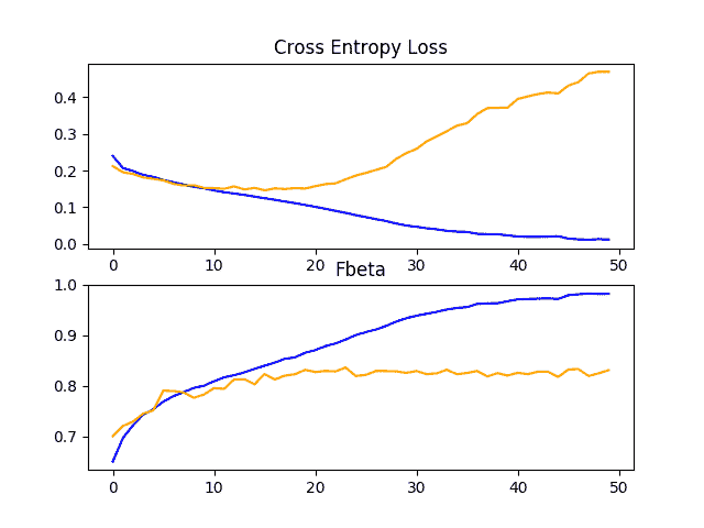
显示列车基线模型和行星问题测试数据集的损失和 F-Beta 学习曲线的线图

既然我们已经有了数据集的基线模型，我们就有了实验和改进的坚实基础。

我们将在下一节探讨一些提高模型表现的想法。

如何提高模型表现

在前一节中，我们定义了一个基线模型，可以作为改进行星数据集的基础。

该模型获得了合理的 F-beta 分数，尽管学习曲线表明该模型过度训练了训练数据集。探索解决过拟合的两种常见方法是丢弃正规化和数据扩充。两者都有破坏和减缓学习过程的效果，特别是模型在训练阶段的改进速度。

我们将在本节中探讨这两种方法。鉴于我们预计学习速度会减慢，我们通过将训练阶段的数量从 50 个增加到 200 个，给模型更多的学习时间。

丢弃正规化

脱落正则化是一种计算量小的正则化深度神经网络的方法。

丢弃的工作原理是从概率上移除，或者“T0”从“T1”中移除，输入到一个层，该层可以是数据样本中的输入变量或者来自前一层的激活。它具有模拟大量具有非常不同的网络结构的网络的效果，并且反过来使得网络中的节点通常对输入更加鲁棒。

有关丢弃的更多信息，请参阅帖子:

• 如何利用 Keras 中的丢弃正则化减少过拟合

通常，每个 VGG 模块后可以施加少量压降，更多压降施加于模型输出层附近的全连接层。

下面是添加了 Dropout 的基线模型的更新版本的 define_model() 函数。在这种情况下，在每个 VGG 块之后应用 20%的丢失率，在模型的分类器部分的完全连接层之后应用更大的 50%的丢失率。

# define cnn model
def define_model(in_shape=(128, 128, 3), out_shape=17):
	model = Sequential()
	model.add(Conv2D(32, (3, 3), activation='relu', kernel_initializer='he_uniform', padding='same', input_shape=in_shape))
	model.add(Conv2D(32, (3, 3), activation='relu', kernel_initializer='he_uniform', padding='same'))
	model.add(MaxPooling2D((2, 2)))
	model.add(Dropout(0.2))
	model.add(Conv2D(64, (3, 3), activation='relu', kernel_initializer='he_uniform', padding='same'))
	model.add(Conv2D(64, (3, 3), activation='relu', kernel_initializer='he_uniform', padding='same'))
	model.add(MaxPooling2D((2, 2)))
	model.add(Dropout(0.2))
	model.add(Conv2D(128, (3, 3), activation='relu', kernel_initializer='he_uniform', padding='same'))
	model.add(Conv2D(128, (3, 3), activation='relu', kernel_initializer='he_uniform', padding='same'))
	model.add(MaxPooling2D((2, 2)))
	model.add(Dropout(0.2))
	model.add(Flatten())
	model.add(Dense(128, activation='relu', kernel_initializer='he_uniform'))
	model.add(Dropout(0.5))
	model.add(Dense(out_shape, activation='sigmoid'))
	# compile model
	opt = SGD(lr=0.01, momentum=0.9)
	model.compile(optimizer=opt, loss='binary_crossentropy', metrics=[fbeta])
	return model

为了完整起见，下面列出了基线模型的完整代码列表，并在行星数据集上添加了 drop。

# baseline model with dropout on the planet dataset
import sys
from numpy import load
from matplotlib import pyplot
from sklearn.model_selection import train_test_split
from keras import backend
from keras.preprocessing.image import ImageDataGenerator
from keras.models import Sequential
from keras.layers import Conv2D
from keras.layers import MaxPooling2D
from keras.layers import Dense
from keras.layers import Flatten
from keras.layers import Dropout
from keras.optimizers import SGD

# load train and test dataset
def load_dataset():
	# load dataset
	data = load('planet_data.npz')
	X, y = data['arr_0'], data['arr_1']
	# separate into train and test datasets
	trainX, testX, trainY, testY = train_test_split(X, y, test_size=0.3, random_state=1)
	print(trainX.shape, trainY.shape, testX.shape, testY.shape)
	return trainX, trainY, testX, testY

# calculate fbeta score for multi-class/label classification
def fbeta(y_true, y_pred, beta=2):
	# clip predictions
	y_pred = backend.clip(y_pred, 0, 1)
	# calculate elements
	tp = backend.sum(backend.round(backend.clip(y_true * y_pred, 0, 1)), axis=1)
	fp = backend.sum(backend.round(backend.clip(y_pred - y_true, 0, 1)), axis=1)
	fn = backend.sum(backend.round(backend.clip(y_true - y_pred, 0, 1)), axis=1)
	# calculate precision
	p = tp / (tp + fp + backend.epsilon())
	# calculate recall
	r = tp / (tp + fn + backend.epsilon())
	# calculate fbeta, averaged across each class
	bb = beta ** 2
	fbeta_score = backend.mean((1 + bb) * (p * r) / (bb * p + r + backend.epsilon()))
	return fbeta_score

# define cnn model
def define_model(in_shape=(128, 128, 3), out_shape=17):
	model = Sequential()
	model.add(Conv2D(32, (3, 3), activation='relu', kernel_initializer='he_uniform', padding='same', input_shape=in_shape))
	model.add(Conv2D(32, (3, 3), activation='relu', kernel_initializer='he_uniform', padding='same'))
	model.add(MaxPooling2D((2, 2)))
	model.add(Dropout(0.2))
	model.add(Conv2D(64, (3, 3), activation='relu', kernel_initializer='he_uniform', padding='same'))
	model.add(Conv2D(64, (3, 3), activation='relu', kernel_initializer='he_uniform', padding='same'))
	model.add(MaxPooling2D((2, 2)))
	model.add(Dropout(0.2))
	model.add(Conv2D(128, (3, 3), activation='relu', kernel_initializer='he_uniform', padding='same'))
	model.add(Conv2D(128, (3, 3), activation='relu', kernel_initializer='he_uniform', padding='same'))
	model.add(MaxPooling2D((2, 2)))
	model.add(Dropout(0.2))
	model.add(Flatten())
	model.add(Dense(128, activation='relu', kernel_initializer='he_uniform'))
	model.add(Dropout(0.5))
	model.add(Dense(out_shape, activation='sigmoid'))
	# compile model
	opt = SGD(lr=0.01, momentum=0.9)
	model.compile(optimizer=opt, loss='binary_crossentropy', metrics=[fbeta])
	return model

# plot diagnostic learning curves
def summarize_diagnostics(history):
	# plot loss
	pyplot.subplot(211)
	pyplot.title('Cross Entropy Loss')
	pyplot.plot(history.history['loss'], color='blue', label='train')
	pyplot.plot(history.history['val_loss'], color='orange', label='test')
	# plot accuracy
	pyplot.subplot(212)
	pyplot.title('Fbeta')
	pyplot.plot(history.history['fbeta'], color='blue', label='train')
	pyplot.plot(history.history['val_fbeta'], color='orange', label='test')
	# save plot to file
	filename = sys.argv[0].split('/')[-1]
	pyplot.savefig(filename + '_plot.png')
	pyplot.close()

# run the test harness for evaluating a model
def run_test_harness():
	# load dataset
	trainX, trainY, testX, testY = load_dataset()
	# create data generator
	datagen = ImageDataGenerator(rescale=1.0/255.0)
	# prepare iterators
	train_it = datagen.flow(trainX, trainY, batch_size=128)
	test_it = datagen.flow(testX, testY, batch_size=128)
	# define model
	model = define_model()
	# fit model
	history = model.fit_generator(train_it, steps_per_epoch=len(train_it),
		validation_data=test_it, validation_steps=len(test_it), epochs=200, verbose=0)
	# evaluate model
	loss, fbeta = model.evaluate_generator(test_it, steps=len(test_it), verbose=0)
	print('> loss=%.3f, fbeta=%.3f' % (loss, fbeta))
	# learning curves
	summarize_diagnostics(history)

# entry point, run the test harness
run_test_harness()

运行该示例首先适合模型，然后在等待测试数据集上报告模型表现。

注:考虑到算法或评估程序的随机性，或数值准确率的差异，您的结果可能会有所不同。考虑运行该示例几次，并比较平均结果。

在这种情况下，我们可以看到模型表现的小幅提升，从基线模型的约 0.831 的 F-beta 分数提升到约 0.859，并增加了脱落。

(28335, 128, 128, 3) (28335, 17) (12144, 128, 128, 3) (12144, 17)
> loss=0.190, fbeta=0.859

回顾学习曲线，我们可以看到丢弃对模型在训练集和测试集上的改进速度有一些影响。

过拟合已经减少或延迟，尽管表现可能会在运行中期开始停滞，大约在纪元 100。

结果表明，可能需要进一步的正规化。这可以通过更大的丢弃率和/或增加重量衰减来实现。此外，批次大小可以减小，学习率可以减小，这两者都可以进一步减缓模型的改进速度，可能对减少训练数据集的过拟合有积极的作用。

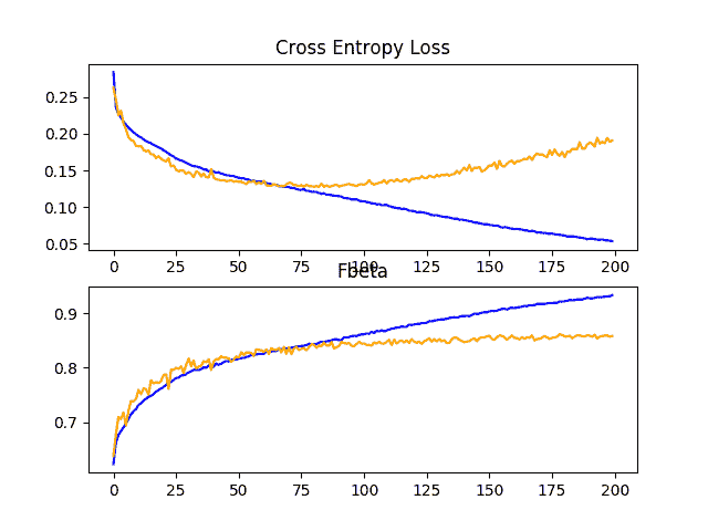
显示列车上有脱落的基线模型和行星问题测试数据集的损失和 F-Beta 学习曲线的线图

图像数据增长

图像数据扩充是一种技术，可用于通过在数据集中创建图像的修改版本来人工扩展训练数据集的大小。

在更多的数据上训练深度学习神经网络模型可以产生更熟练的模型，并且增强技术可以创建图像的变化，这可以提高拟合模型将他们所学知识推广到新图像的能力。

数据扩充也可以作为一种正则化技术，向训练数据添加噪声，并鼓励模型学习相同的特征，这些特征在输入中的位置是不变的。

对卫星照片的输入照片进行小的更改可能对解决这个问题有用，例如水平翻转、垂直翻转、旋转、缩放，也许还有更多。这些扩充可以被指定为用于训练数据集的图像数据生成器实例的参数。增强不应用于测试数据集，因为我们希望在未修改的照片上评估模型的表现。

这要求我们为训练和测试数据集有一个单独的 ImageDataGenerator 实例，然后为从各自的数据生成器创建的训练和测试集有迭代器。例如:

# create data generator
train_datagen = ImageDataGenerator(rescale=1.0/255.0, horizontal_flip=True, vertical_flip=True, rotation_range=90)
test_datagen = ImageDataGenerator(rescale=1.0/255.0)
# prepare iterators
train_it = train_datagen.flow(trainX, trainY, batch_size=128)
test_it = test_datagen.flow(testX, testY, batch_size=128)

在这种情况下，训练数据集中的照片将通过随机水平和垂直翻转以及高达 90 度的随机旋转来增强。在训练和测试步骤中，照片的像素值将按照与基线模型相同的方式进行缩放。

为了完整起见，下面列出了带有行星数据集训练数据扩充的基线模型的完整代码列表。

# baseline model with data augmentation for the planet dataset
import sys
from numpy import load
from matplotlib import pyplot
from sklearn.model_selection import train_test_split
from keras import backend
from keras.preprocessing.image import ImageDataGenerator
from keras.models import Sequential
from keras.layers import Conv2D
from keras.layers import MaxPooling2D
from keras.layers import Dense
from keras.layers import Flatten
from keras.optimizers import SGD

# load train and test dataset
def load_dataset():
	# load dataset
	data = load('planet_data.npz')
	X, y = data['arr_0'], data['arr_1']
	# separate into train and test datasets
	trainX, testX, trainY, testY = train_test_split(X, y, test_size=0.3, random_state=1)
	print(trainX.shape, trainY.shape, testX.shape, testY.shape)
	return trainX, trainY, testX, testY

# calculate fbeta score for multi-class/label classification
def fbeta(y_true, y_pred, beta=2):
	# clip predictions
	y_pred = backend.clip(y_pred, 0, 1)
	# calculate elements
	tp = backend.sum(backend.round(backend.clip(y_true * y_pred, 0, 1)), axis=1)
	fp = backend.sum(backend.round(backend.clip(y_pred - y_true, 0, 1)), axis=1)
	fn = backend.sum(backend.round(backend.clip(y_true - y_pred, 0, 1)), axis=1)
	# calculate precision
	p = tp / (tp + fp + backend.epsilon())
	# calculate recall
	r = tp / (tp + fn + backend.epsilon())
	# calculate fbeta, averaged across each class
	bb = beta ** 2
	fbeta_score = backend.mean((1 + bb) * (p * r) / (bb * p + r + backend.epsilon()))
	return fbeta_score

# define cnn model
def define_model(in_shape=(128, 128, 3), out_shape=17):
	model = Sequential()
	model.add(Conv2D(32, (3, 3), activation='relu', kernel_initializer='he_uniform', padding='same', input_shape=in_shape))
	model.add(Conv2D(32, (3, 3), activation='relu', kernel_initializer='he_uniform', padding='same'))
	model.add(MaxPooling2D((2, 2)))
	model.add(Conv2D(64, (3, 3), activation='relu', kernel_initializer='he_uniform', padding='same'))
	model.add(Conv2D(64, (3, 3), activation='relu', kernel_initializer='he_uniform', padding='same'))
	model.add(MaxPooling2D((2, 2)))
	model.add(Conv2D(128, (3, 3), activation='relu', kernel_initializer='he_uniform', padding='same'))
	model.add(Conv2D(128, (3, 3), activation='relu', kernel_initializer='he_uniform', padding='same'))
	model.add(MaxPooling2D((2, 2)))
	model.add(Flatten())
	model.add(Dense(128, activation='relu', kernel_initializer='he_uniform'))
	model.add(Dense(out_shape, activation='sigmoid'))
	# compile model
	opt = SGD(lr=0.01, momentum=0.9)
	model.compile(optimizer=opt, loss='binary_crossentropy', metrics=[fbeta])
	return model

# plot diagnostic learning curves
def summarize_diagnostics(history):
	# plot loss
	pyplot.subplot(211)
	pyplot.title('Cross Entropy Loss')
	pyplot.plot(history.history['loss'], color='blue', label='train')
	pyplot.plot(history.history['val_loss'], color='orange', label='test')
	# plot accuracy
	pyplot.subplot(212)
	pyplot.title('Fbeta')
	pyplot.plot(history.history['fbeta'], color='blue', label='train')
	pyplot.plot(history.history['val_fbeta'], color='orange', label='test')
	# save plot to file
	filename = sys.argv[0].split('/')[-1]
	pyplot.savefig(filename + '_plot.png')
	pyplot.close()

# run the test harness for evaluating a model
def run_test_harness():
	# load dataset
	trainX, trainY, testX, testY = load_dataset()
	# create data generator
	train_datagen = ImageDataGenerator(rescale=1.0/255.0, horizontal_flip=True, vertical_flip=True, rotation_range=90)
	test_datagen = ImageDataGenerator(rescale=1.0/255.0)
	# prepare iterators
	train_it = train_datagen.flow(trainX, trainY, batch_size=128)
	test_it = test_datagen.flow(testX, testY, batch_size=128)
	# define model
	model = define_model()
	# fit model
	history = model.fit_generator(train_it, steps_per_epoch=len(train_it),
		validation_data=test_it, validation_steps=len(test_it), epochs=200, verbose=0)
	# evaluate model
	loss, fbeta = model.evaluate_generator(test_it, steps=len(test_it), verbose=0)
	print('> loss=%.3f, fbeta=%.3f' % (loss, fbeta))
	# learning curves
	summarize_diagnostics(history)

# entry point, run the test harness
run_test_harness()

运行该示例首先适合模型，然后在等待测试数据集上报告模型表现。

注:考虑到算法或评估程序的随机性，或数值准确率的差异，您的结果可能会有所不同。考虑运行该示例几次，并比较平均结果。

在这种情况下，我们可以看到表现提升了大约 0.06，从基线模型的大约 0.831 的 F-beta 分数提升到具有简单数据增加的基线模型的大约 0.882 的分数。这是一个很大的进步，比我们看到的丢弃率要大。

(28335, 128, 128, 3) (28335, 17) (12144, 128, 128, 3) (12144, 17)
> loss=0.103, fbeta=0.882

回顾学习曲线，我们可以看到过拟合受到了巨大的影响。学习一直持续到 100 年以后，尽管可能会在跑步结束时显示出趋于平稳的迹象。结果表明，进一步增强或其他类型的正则化添加到这种配置可能会有所帮助。

探索额外的图像扩充可能会很有意思，这些图像扩充可以进一步鼓励学习对其在输入中的位置不变的特征，例如缩放和移位。

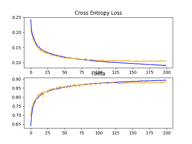
显示基线模型的损失和 F-Beta 学习曲线的线图，在行星问题的训练和测试数据集上有数据增加

讨论

我们对基线模型进行了两种不同的改进。

结果可以总结如下，尽管我们必须假设这些结果中存在一些方差，因为算法具有随机性:

• 基线+丢弃正规化 : 0.859
• 基线+数据增加 : 0.882

正如所怀疑的那样，正则化技术的加入减缓了学习算法的进程，减少了过拟合，从而提高了保持数据集的表现。这两种方法的结合以及训练期数量的进一步增加很可能会带来进一步的改进。也就是说，丢弃和数据增加的结合。

这只是可以在这个数据集上探索的改进类型的开始。除了对所描述的正则化方法进行调整之外，还可以探索其他正则化方法，例如权重衰减和提前停止。

探索学习算法的变化可能是值得的，例如学习率的变化、学习率时间表的使用或自适应学习率，如 Adam。

替代模型架构也值得探索。所选的基准模型预计会提供比解决此问题所需的更多的容量，较小的模型可能会更快地进行训练，从而提高表现。

如何运用迁移学习

迁移学习涉及使用在相关任务上训练的模型的全部或部分。

Keras 提供了一系列预先训练好的模型，可以通过 Keras 应用 API 全部或部分加载和使用。

迁移学习的一个有用模型是 VGG 模型之一，例如具有 16 层的 VGG-16，在开发时，它在 ImageNet 照片分类挑战中取得了顶级表现。

该模型由两个主要部分组成:由 VGG 块组成的模型的特征提取器部分，以及由完全连接的层和输出层组成的模型的分类器部分。

我们可以使用模型的特征提取部分，并添加一个新的分类器部分的模型，这是量身定制的行星数据集。具体来说，我们可以在训练过程中保持所有卷积层的权重固定，并且只训练新的完全连接的层，这些层将学习解释从模型中提取的特征，并进行一套二进制分类。

这可以通过加载 VGG-16 模型，从模型的输出端移除全连接层，然后添加新的全连接层来解释模型输出并进行预测来实现。通过将“ include_top ”参数设置为“ False ，可以自动移除模型的分类器部分，这也要求为模型指定输入的形状，在本例中为(128，128，3)。这意味着加载的模型在最后一个最大池层结束，之后我们可以手动添加一个扁平化层和新的分类器全连接层。

下面的 define_model() 函数实现了这一点，并返回一个准备训练的新模型。

# define cnn model
def define_model(in_shape=(128, 128, 3), out_shape=17):
	# load model
	model = VGG16(include_top=False, input_shape=in_shape)
	# mark loaded layers as not trainable
	for layer in model.layers:
		layer.trainable = False
	# add new classifier layers
	flat1 = Flatten()(model.layers[-1].output)
	class1 = Dense(128, activation='relu', kernel_initializer='he_uniform')(flat1)
	output = Dense(out_shape, activation='sigmoid')(class1)
	# define new model
	model = Model(inputs=model.inputs, outputs=output)
	# compile model
	opt = SGD(lr=0.01, momentum=0.9)
	model.compile(optimizer=opt, loss='binary_crossentropy', metrics=[fbeta])
	return model

一旦创建，我们就可以像以前一样在训练数据集上训练模型。

在这种情况下，不需要大量的训练，因为只有新的完全连接和输出层具有可训练的权重。因此，我们将把训练时期的数量固定在 10 个。

VGG16 模型在特定的 ImageNet 挑战数据集上进行了训练。因此，模型期望图像居中。也就是说，从输入中减去在 ImageNet 训练数据集上计算的每个通道(红色、绿色和蓝色)的平均像素值。

Keras 通过*预处理 _ 输入()*功能提供了一个为单个照片执行该准备的功能。尽管如此，通过将“ featurewise_center ”参数设置为“ True ”并手动指定居中时使用的平均像素值作为来自 ImageNet 训练数据集的平均值，我们可以使用图像数据生成器实现相同的效果:[123.68，116.779，103.939]。

# create data generator
datagen = ImageDataGenerator(featurewise_center=True)
# specify imagenet mean values for centering
datagen.mean = [123.68, 116.779, 103.939]

下面列出了行星数据集上用于转移学习的 VGG-16 模型的完整代码列表。

# vgg16 transfer learning on the planet dataset
import sys
from numpy import load
from matplotlib import pyplot
from sklearn.model_selection import train_test_split
from keras import backend
from keras.layers import Dense
from keras.layers import Flatten
from keras.optimizers import SGD
from keras.applications.vgg16 import VGG16
from keras.models import Model
from keras.preprocessing.image import ImageDataGenerator

# load train and test dataset
def load_dataset():
	# load dataset
	data = load('planet_data.npz')
	X, y = data['arr_0'], data['arr_1']
	# separate into train and test datasets
	trainX, testX, trainY, testY = train_test_split(X, y, test_size=0.3, random_state=1)
	print(trainX.shape, trainY.shape, testX.shape, testY.shape)
	return trainX, trainY, testX, testY

# calculate fbeta score for multi-class/label classification
def fbeta(y_true, y_pred, beta=2):
	# clip predictions
	y_pred = backend.clip(y_pred, 0, 1)
	# calculate elements
	tp = backend.sum(backend.round(backend.clip(y_true * y_pred, 0, 1)), axis=1)
	fp = backend.sum(backend.round(backend.clip(y_pred - y_true, 0, 1)), axis=1)
	fn = backend.sum(backend.round(backend.clip(y_true - y_pred, 0, 1)), axis=1)
	# calculate precision
	p = tp / (tp + fp + backend.epsilon())
	# calculate recall
	r = tp / (tp + fn + backend.epsilon())
	# calculate fbeta, averaged across each class
	bb = beta ** 2
	fbeta_score = backend.mean((1 + bb) * (p * r) / (bb * p + r + backend.epsilon()))
	return fbeta_score

# define cnn model
def define_model(in_shape=(128, 128, 3), out_shape=17):
	# load model
	model = VGG16(include_top=False, input_shape=in_shape)
	# mark loaded layers as not trainable
	for layer in model.layers:
		layer.trainable = False
	# add new classifier layers
	flat1 = Flatten()(model.layers[-1].output)
	class1 = Dense(128, activation='relu', kernel_initializer='he_uniform')(flat1)
	output = Dense(out_shape, activation='sigmoid')(class1)
	# define new model
	model = Model(inputs=model.inputs, outputs=output)
	# compile model
	opt = SGD(lr=0.01, momentum=0.9)
	model.compile(optimizer=opt, loss='binary_crossentropy', metrics=[fbeta])
	return model

# plot diagnostic learning curves
def summarize_diagnostics(history):
	# plot loss
	pyplot.subplot(211)
	pyplot.title('Cross Entropy Loss')
	pyplot.plot(history.history['loss'], color='blue', label='train')
	pyplot.plot(history.history['val_loss'], color='orange', label='test')
	# plot accuracy
	pyplot.subplot(212)
	pyplot.title('Fbeta')
	pyplot.plot(history.history['fbeta'], color='blue', label='train')
	pyplot.plot(history.history['val_fbeta'], color='orange', label='test')
	# save plot to file
	filename = sys.argv[0].split('/')[-1]
	pyplot.savefig(filename + '_plot.png')
	pyplot.close()

# run the test harness for evaluating a model
def run_test_harness():
	# load dataset
	trainX, trainY, testX, testY = load_dataset()
	# create data generator
	datagen = ImageDataGenerator(featurewise_center=True)
	# specify imagenet mean values for centering
	datagen.mean = [123.68, 116.779, 103.939]
	# prepare iterators
	train_it = datagen.flow(trainX, trainY, batch_size=128)
	test_it = datagen.flow(testX, testY, batch_size=128)
	# define model
	model = define_model()
	# fit model
	history = model.fit_generator(train_it, steps_per_epoch=len(train_it),
		validation_data=test_it, validation_steps=len(test_it), epochs=20, verbose=0)
	# evaluate model
	loss, fbeta = model.evaluate_generator(test_it, steps=len(test_it), verbose=0)
	print('> loss=%.3f, fbeta=%.3f' % (loss, fbeta))
	# learning curves
	summarize_diagnostics(history)

# entry point, run the test harness
run_test_harness()

运行该示例首先适合模型，然后在等待测试数据集上报告模型表现。

注:考虑到算法或评估程序的随机性，或数值准确率的差异，您的结果可能会有所不同。考虑运行该示例几次，并比较平均结果。

在这种情况下，我们可以看到该模型获得了约 0.860 的 F-beta 评分，优于基线模型，但不如具有图像数据扩充的基线模型。

(28335, 128, 128, 3) (28335, 17) (12144, 128, 128, 3) (12144, 17)
> loss=0.152, fbeta=0.860

回顾学习曲线，我们可以看到模型很快拟合数据集，仅在几个训练时期内就显示出很强的过拟合。

结果表明，该模型可以受益于正则化，以解决过拟合，并可能对模型或学习过程进行其他更改，以减缓改进速度。

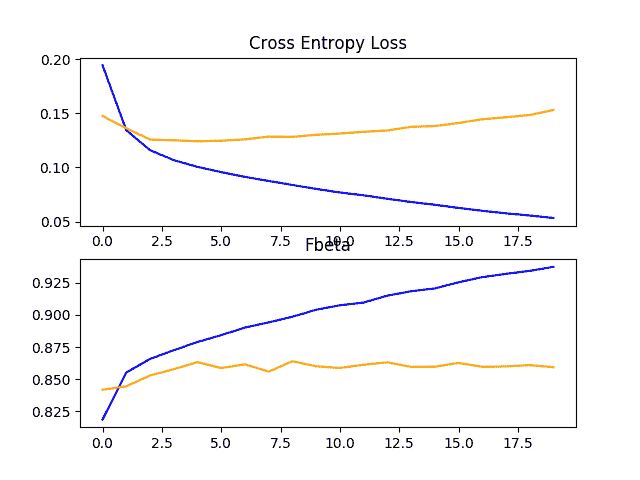
在行星问题的训练和测试数据集上显示 VGG-16 模型的损失和 F-Beta 学习曲线的线图

VGG-16 模型旨在将对象照片分为 1000 个类别之一。因此，它被设计来挑选对象的细粒度特征。我们可以猜测，模型通过更深层学习到的特征将代表 ImageNet 数据集中看到的高阶特征，这些特征可能与亚马逊雨林卫星照片的分类没有直接关系。

为了解决这个问题，我们可以重新拟合 VGG-16 模型，并允许训练算法微调模型中某些层的权重。在这种情况下，我们将使三个卷积层(和一致性池层)成为可训练的。下面列出了 define_model() 功能的更新版本。

# define cnn model
def define_model(in_shape=(128, 128, 3), out_shape=17):
	# load model
	model = VGG16(include_top=False, input_shape=in_shape)
	# mark loaded layers as not trainable
	for layer in model.layers:
		layer.trainable = False
	# allow last vgg block to be trainable
	model.get_layer('block5_conv1').trainable = True
	model.get_layer('block5_conv2').trainable = True
	model.get_layer('block5_conv3').trainable = True
	model.get_layer('block5_pool').trainable = True
	# add new classifier layers
	flat1 = Flatten()(model.layers[-1].output)
	class1 = Dense(128, activation='relu', kernel_initializer='he_uniform')(flat1)
	output = Dense(out_shape, activation='sigmoid')(class1)
	# define new model
	model = Model(inputs=model.inputs, outputs=output)
	# compile model
	opt = SGD(lr=0.01, momentum=0.9)
	model.compile(optimizer=opt, loss='binary_crossentropy', metrics=[fbeta])

然后，在行星数据集上使用 VGG-16 的转移学习的例子可以通过这种修改重新运行。

注:考虑到算法或评估程序的随机性，或数值准确率的差异，您的结果可能会有所不同。考虑运行该示例几次，并比较平均结果。

在这种情况下，我们看到，与 VGG-16 模型特征提取模型相比，模型表现有所提高，因为它将 F-beta 评分从约 0.860 提高到约 0.879。该分数接近基线模型的 F-beta 分数，增加了图像数据扩充。

(28335, 128, 128, 3) (28335, 17) (12144, 128, 128, 3) (12144, 17)
> loss=0.210, fbeta=0.879

回顾学习曲线，我们可以看到模型在运行的相对早期仍然显示出过拟合训练数据集的迹象。结果表明，也许该模型可以受益于丢弃和/或其他正则化方法的使用。

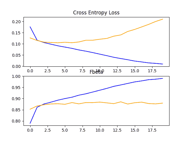
鉴于我们看到在基线模型上使用数据扩充有了很大的改进，我们可能有兴趣看看数据扩充是否可以通过微调来提高 VGG-16 模型的表现。

在这种情况下，可以使用相同的 define_model() 功能，尽管在这种情况下可以更新*run _ test _ 线束()*以使用上一节中执行的图像数据扩充。我们预计增加数据增加将减缓改进速度。因此，我们将把训练阶段的数量从 20 个增加到 50 个，以便让模型有更多的时间收敛。

带有微调和数据扩充的 VGG-16 的完整例子如下。

# vgg with fine-tuning and data augmentation for the planet dataset
import sys
from numpy import load
from matplotlib import pyplot
from sklearn.model_selection import train_test_split
from keras import backend
from keras.layers import Dense
from keras.layers import Flatten
from keras.optimizers import SGD
from keras.applications.vgg16 import VGG16
from keras.models import Model
from keras.preprocessing.image import ImageDataGenerator

# load train and test dataset
def load_dataset():
	# load dataset
	data = load('planet_data.npz')
	X, y = data['arr_0'], data['arr_1']
	# separate into train and test datasets
	trainX, testX, trainY, testY = train_test_split(X, y, test_size=0.3, random_state=1)
	print(trainX.shape, trainY.shape, testX.shape, testY.shape)
	return trainX, trainY, testX, testY

# calculate fbeta score for multi-class/label classification
def fbeta(y_true, y_pred, beta=2):
	# clip predictions
	y_pred = backend.clip(y_pred, 0, 1)
	# calculate elements
	tp = backend.sum(backend.round(backend.clip(y_true * y_pred, 0, 1)), axis=1)
	fp = backend.sum(backend.round(backend.clip(y_pred - y_true, 0, 1)), axis=1)
	fn = backend.sum(backend.round(backend.clip(y_true - y_pred, 0, 1)), axis=1)
	# calculate precision
	p = tp / (tp + fp + backend.epsilon())
	# calculate recall
	r = tp / (tp + fn + backend.epsilon())
	# calculate fbeta, averaged across each class
	bb = beta ** 2
	fbeta_score = backend.mean((1 + bb) * (p * r) / (bb * p + r + backend.epsilon()))
	return fbeta_score

# define cnn model
def define_model(in_shape=(128, 128, 3), out_shape=17):
	# load model
	model = VGG16(include_top=False, input_shape=in_shape)
	# mark loaded layers as not trainable
	for layer in model.layers:
		layer.trainable = False
	# allow last vgg block to be trainable
	model.get_layer('block5_conv1').trainable = True
	model.get_layer('block5_conv2').trainable = True
	model.get_layer('block5_conv3').trainable = True
	model.get_layer('block5_pool').trainable = True
	# add new classifier layers
	flat1 = Flatten()(model.layers[-1].output)
	class1 = Dense(128, activation='relu', kernel_initializer='he_uniform')(flat1)
	output = Dense(out_shape, activation='sigmoid')(class1)
	# define new model
	model = Model(inputs=model.inputs, outputs=output)
	# compile model
	opt = SGD(lr=0.01, momentum=0.9)
	model.compile(optimizer=opt, loss='binary_crossentropy', metrics=[fbeta])
	return model

# plot diagnostic learning curves
def summarize_diagnostics(history):
	# plot loss
	pyplot.subplot(211)
	pyplot.title('Cross Entropy Loss')
	pyplot.plot(history.history['loss'], color='blue', label='train')
	pyplot.plot(history.history['val_loss'], color='orange', label='test')
	# plot accuracy
	pyplot.subplot(212)
	pyplot.title('Fbeta')
	pyplot.plot(history.history['fbeta'], color='blue', label='train')
	pyplot.plot(history.history['val_fbeta'], color='orange', label='test')
	# save plot to file
	filename = sys.argv[0].split('/')[-1]
	pyplot.savefig(filename + '_plot.png')
	pyplot.close()

# run the test harness for evaluating a model
def run_test_harness():
	# load dataset
	trainX, trainY, testX, testY = load_dataset()
	# create data generator
	train_datagen = ImageDataGenerator(featurewise_center=True, horizontal_flip=True, vertical_flip=True, rotation_range=90)
	test_datagen = ImageDataGenerator(featurewise_center=True)
	# specify imagenet mean values for centering
	train_datagen.mean = [123.68, 116.779, 103.939]
	test_datagen.mean = [123.68, 116.779, 103.939]
	# prepare iterators
	train_it = train_datagen.flow(trainX, trainY, batch_size=128)
	test_it = test_datagen.flow(testX, testY, batch_size=128)
	# define model
	model = define_model()
	# fit model
	history = model.fit_generator(train_it, steps_per_epoch=len(train_it),
		validation_data=test_it, validation_steps=len(test_it), epochs=50, verbose=0)
	# evaluate model
	loss, fbeta = model.evaluate_generator(test_it, steps=len(test_it), verbose=0)
	print('> loss=%.3f, fbeta=%.3f' % (loss, fbeta))
	# learning curves
	summarize_diagnostics(history)

# entry point, run the test harness
run_test_harness()

运行该示例首先适合模型，然后在等待测试数据集上报告模型表现。

注:考虑到算法或评估程序的随机性，或数值准确率的差异，您的结果可能会有所不同。考虑运行该示例几次，并比较平均结果。

在这种情况下，我们可以看到模型表现从大约 0.879 的 F-beta 分数进一步提升到大约 0.891 的 F-beta 分数。

(28335, 128, 128, 3) (28335, 17) (12144, 128, 128, 3) (12144, 17)
> loss=0.100, fbeta=0.891

回顾学习曲线，我们可以看到数据扩充再次对模型过拟合产生了很大的影响，在这种情况下，稳定学习并延迟过拟合可能直到 20 世纪。

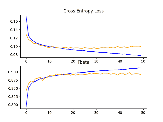
显示 VGG-16 模型的损失和 F-Beta 学习曲线的线图，在行星问题的训练和测试数据集上进行了微调和数据扩充

讨论

在本节中，我们探讨了三种不同的迁移学习案例

结果可以总结如下，尽管我们必须假设这些结果中存在一些方差，因为学习算法具有随机性:

• 墙-16 型 : 0.860。
• VGG-16 车型+微调 : 0.879。
• VGG-16 型号+微调+数据扩充 : 0.891。

VGG-16 型号的选择有些武断，因为它是一个较小的、众所周知的型号。其他模型可以作为迁移学习的基础，如 ResNet ，可能会取得更好的表现。

此外，更多的微调也可能导致更好的表现。这可能包括调整更多特征提取器层的权重，可能学习率更低。这也可能包括修改模型以增加正则化，如丢弃。

如何最终确定模型并做出预测

只要我们有想法，有时间和资源来测试，模型改进的过程可能会持续很长时间。

在某些时候，必须选择并采用最终的模型配置。在这种情况下，我们将保持事情简单，并使用 VGG-16 转移学习，微调和数据增加作为最终模型。

首先，我们将通过在整个训练数据集上拟合模型并将模型保存到文件中以备后用来最终确定我们的模型。然后，我们将加载保存的模型，并使用它对单个图像进行预测。

保存最终模型

第一步是在整个训练数据集上拟合最终模型。

可以更新 load_dataset() 函数，不再将加载的数据集拆分为训练集和测试集。

# load train and test dataset
def load_dataset():
	# load dataset
	data = load('planet_data.npz')
	X, y = data['arr_0'], data['arr_1']
	return X, y

define_model() 函数可以像上一节中为 VGG-16 模型定义的那样使用，具有微调和数据扩充功能。

# define cnn model
def define_model(in_shape=(128, 128, 3), out_shape=17):
	# load model
	model = VGG16(include_top=False, input_shape=in_shape)
	# mark loaded layers as not trainable
	for layer in model.layers:
		layer.trainable = False
	# allow last vgg block to be trainable
	model.get_layer('block5_conv1').trainable = True
	model.get_layer('block5_conv2').trainable = True
	model.get_layer('block5_conv3').trainable = True
	model.get_layer('block5_pool').trainable = True
	# add new classifier layers
	flat1 = Flatten()(model.layers[-1].output)
	class1 = Dense(128, activation='relu', kernel_initializer='he_uniform')(flat1)
	output = Dense(out_shape, activation='sigmoid')(class1)
	# define new model
	model = Model(inputs=model.inputs, outputs=output)
	# compile model
	opt = SGD(lr=0.01, momentum=0.9)
	model.compile(optimizer=opt, loss='binary_crossentropy')
	return model

最后，对于训练数据集，我们只需要一个数据生成器和一个迭代器。

# create data generator
datagen = ImageDataGenerator(featurewise_center=True, horizontal_flip=True, vertical_flip=True, rotation_range=90)
# specify imagenet mean values for centering
datagen.mean = [123.68, 116.779, 103.939]
# prepare iterator
train_it = datagen.flow(X, y, batch_size=128)

该模型将适用于 50 个时代，之后将通过调用模型上的 save() 函数将其保存到 H5 文件中

# fit model
model.fit_generator(train_it, steps_per_epoch=len(train_it), epochs=50, verbose=0)
# save model
model.save('final_model.h5')

注意:保存和加载 Keras 模型需要在您的工作站上安装 h5py 库。

下面列出了在训练数据集上拟合最终模型并将其保存到文件中的完整示例。

# save the final model to file
from numpy import load
from keras.preprocessing.image import ImageDataGenerator
from keras.applications.vgg16 import VGG16
from keras.models import Model
from keras.layers import Dense
from keras.layers import Flatten
from keras.optimizers import SGD

# load train and test dataset
def load_dataset():
	# load dataset
	data = load('planet_data.npz')
	X, y = data['arr_0'], data['arr_1']
	return X, y

# define cnn model
def define_model(in_shape=(128, 128, 3), out_shape=17):
	# load model
	model = VGG16(include_top=False, input_shape=in_shape)
	# mark loaded layers as not trainable
	for layer in model.layers:
		layer.trainable = False
	# allow last vgg block to be trainable
	model.get_layer('block5_conv1').trainable = True
	model.get_layer('block5_conv2').trainable = True
	model.get_layer('block5_conv3').trainable = True
	model.get_layer('block5_pool').trainable = True
	# add new classifier layers
	flat1 = Flatten()(model.layers[-1].output)
	class1 = Dense(128, activation='relu', kernel_initializer='he_uniform')(flat1)
	output = Dense(out_shape, activation='sigmoid')(class1)
	# define new model
	model = Model(inputs=model.inputs, outputs=output)
	# compile model
	opt = SGD(lr=0.01, momentum=0.9)
	model.compile(optimizer=opt, loss='binary_crossentropy')
	return model

# run the test harness for evaluating a model
def run_test_harness():
	# load dataset
	X, y = load_dataset()
	# create data generator
	datagen = ImageDataGenerator(featurewise_center=True, horizontal_flip=True, vertical_flip=True, rotation_range=90)
	# specify imagenet mean values for centering
	datagen.mean = [123.68, 116.779, 103.939]
	# prepare iterator
	train_it = datagen.flow(X, y, batch_size=128)
	# define model
	model = define_model()
	# fit model
	model.fit_generator(train_it, steps_per_epoch=len(train_it), epochs=50, verbose=0)
	# save model
	model.save('final_model.h5')

# entry point, run the test harness
run_test_harness()

运行此示例后，您将在当前工作目录中拥有一个名为“final_model.h5”的 91 兆字节大文件。

做个预测

我们可以使用保存的模型对新图像进行预测。

该模型假设新图像是彩色的，并且它们已经被分割成大小为 256×256 的正方形。

下面是从训练数据集中提取的图像，具体是文件 train_1.jpg 。

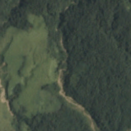
亚马逊雨林卫星图像样本用于预测

将其从您的训练数据目录复制到当前工作目录，名称为“ sample_image.jpg ，例如:

cp train-jpg/train_1.jpg ./sample_image.jpg

根据训练数据集的映射文件，该文件具有以下标记(没有特定的顺序):

• 农业
• 清楚的
• 主要的
• 水

我们将假装这是一个全新的、看不见的图像，按照要求的方式准备，并看看我们如何使用保存的模型来预测图像所代表的标签。

首先，我们可以加载图像，并强制其大小为 128×128 像素。然后可以调整加载图像的大小，使其在数据集中具有单个样本。像素值也必须居中，以匹配模型训练期间准备数据的方式。

load_image() 函数实现了这一点，并将返回已加载的准备分类的图像。

# load and prepare the image
def load_image(filename):
	# load the image
	img = load_img(filename, target_size=(128, 128))
	# convert to array
	img = img_to_array(img)
	# reshape into a single sample with 3 channels
	img = img.reshape(1, 128, 128, 3)
	# center pixel data
	img = img.astype('float32')
	img = img - [123.68, 116.779, 103.939]
	return img

接下来，我们可以像上一节一样加载模型，并调用 predict() 函数来预测图像中的内容。

# predict the class
result = model.predict(img)

这将返回一个浮点值介于 0 和 1 之间的 17 元素向量，该向量可以解释为模型相信照片可以用每个已知标签进行标记的概率。

我们可以将这些概率取整为 0 或 1，然后使用我们在第一部分 create_tag_mapping() 函数中准备的反向映射，将具有“ 1 值的向量索引转换为图像的标签。

下面的 prediction_to_tags() 函数实现了这一点，取整数到标签和模型为照片预测的向量的逆映射，返回预测标签列表。

# convert a prediction to tags
def prediction_to_tags(inv_mapping, prediction):
	# round probabilities to {0, 1}
	values = prediction.round()
	# collect all predicted tags
	tags = [inv_mapping[i] for i in range(len(values)) if values[i] == 1.0]
	return tags

我们可以把这些联系起来，对新照片做出预测。下面列出了完整的示例。

# make a prediction for a new image
from pandas import read_csv
from keras.preprocessing.image import load_img
from keras.preprocessing.image import img_to_array
from keras.models import load_model

# create a mapping of tags to integers given the loaded mapping file
def create_tag_mapping(mapping_csv):
	# create a set of all known tags
	labels = set()
	for i in range(len(mapping_csv)):
		# convert spaced separated tags into an array of tags
		tags = mapping_csv['tags'][i].split(' ')
		# add tags to the set of known labels
		labels.update(tags)
	# convert set of labels to a list to list
	labels = list(labels)
	# order set alphabetically
	labels.sort()
	# dict that maps labels to integers, and the reverse
	labels_map = {labels[i]:i for i in range(len(labels))}
	inv_labels_map = {i:labels[i] for i in range(len(labels))}
	return labels_map, inv_labels_map

# convert a prediction to tags
def prediction_to_tags(inv_mapping, prediction):
	# round probabilities to {0, 1}
	values = prediction.round()
	# collect all predicted tags
	tags = [inv_mapping[i] for i in range(len(values)) if values[i] == 1.0]
	return tags

# load and prepare the image
def load_image(filename):
	# load the image
	img = load_img(filename, target_size=(128, 128))
	# convert to array
	img = img_to_array(img)
	# reshape into a single sample with 3 channels
	img = img.reshape(1, 128, 128, 3)
	# center pixel data
	img = img.astype('float32')
	img = img - [123.68, 116.779, 103.939]
	return img

# load an image and predict the class
def run_example(inv_mapping):
	# load the image
	img = load_image('sample_image.jpg')
	# load model
	model = load_model('final_model.h5')
	# predict the class
	result = model.predict(img)
	print(result[0])
	# map prediction to tags
	tags = prediction_to_tags(inv_mapping, result[0])
	print(tags)

# load the mapping file
filename = 'train_v2.csv'
mapping_csv = read_csv(filename)
# create a mapping of tags to integers
_, inv_mapping = create_tag_mapping(mapping_csv)
# entry point, run the example
run_example(inv_mapping)

运行该示例首先加载和准备图像，加载模型，然后进行预测。

首先，打印原始的 17 元素预测向量。如果我们愿意，我们可以漂亮地打印这个向量，并总结照片将被分配每个标签的预测置信度。

接下来，对预测进行舍入，并将包含 1 值的向量索引反向映射到它们的标记字符串值。然后打印预测的标签。我们可以看到，该模型已经正确预测了所提供照片的已知标签。

在您已经手动建议了标签之后，用一张全新的照片(例如测试数据集中的照片)重复这个测试可能会很有趣。

[9.0940112e-01 3.6541668e-03 1.5959743e-02 6.8241461e-05 8.5694155e-05
 9.9828100e-01 7.4096164e-08 5.5998818e-05 3.6668104e-01 1.2538023e-01
 4.6371704e-04 3.7660234e-04 9.9999273e-01 1.9014676e-01 5.6060363e-04
 1.4613305e-03 9.5227945e-01]

['agriculture', 'clear', 'primary', 'water']

扩展ˌ扩张

本节列出了一些您可能希望探索的扩展教程的想法。

• 调整学习率。探索对用于训练基线模型的学习算法的更改，例如替代学习率、学习率计划或自适应学习率算法，例如 Adam。
• 正则化迁移学习模型。探索在迁移学习中添加进一步的正则化技术，如提前停止、退出、权重衰减等，并比较结果。
• 测试时间自动化。更新模型以使用测试时间预测，例如翻转、旋转和/或裁剪，以查看测试数据集上的预测表现是否可以进一步提高。

如果你探索这些扩展，我很想知道。
在下面的评论中发表你的发现。

进一步阅读

如果您想了解得更深入，本节将提供关于该主题的更多资源。

应用程序接口

• 喀拉拉形象有用的源代码。
• Keras 应用程序接口
• Keras 图像处理 API
• Keras 顺序模型 API
• 硬化. metrics.fbeta_score.html API
• sklearn . model _ selection . train _ test _ split API
• 旧版本的 Keras 指标源代码(带 fbeta_score)。
• Keras、卡格尔内核的 F-beta 评分。

文章

• 星球:从太空了解亚马逊，卡格尔竞赛。
• 下载星球数据集，卡格尔。
• 星球竞赛模型评估，卡格尔。
• 星球:从太空了解亚马逊，第一名得主访谈，2017。
• f1 得分，维基百科
• 精准与召回，维基百科。

摘要

在本教程中，您发现了如何开发卷积神经网络来对亚马逊热带雨林的卫星照片进行分类。

具体来说，您了解到:

• 如何加载准备亚马逊热带雨林卫星照片进行建模？
• 如何从零开始开发卷积神经网络进行照片分类并提高模型表现？
• 如何开发最终模型，并使用它对新数据进行特别预测。

你有什么问题吗？
在下面的评论中提问，我会尽力回答。*