


如何从零开始为 CIFAR-10 照片分类开发 CNN
最后更新于 2020 年 8 月 28 日
了解如何为 CIFAR-10 对象类别数据集从头开发深度卷积神经网络模型。
CIFAR-10 小照片分类问题是计算机视觉和深度学习中使用的标准数据集。
虽然数据集得到了有效解决,但它可以作为学习和实践如何从零开始开发、评估和使用卷积深度学习神经网络进行图像分类的基础。
这包括如何开发一个健壮的测试工具来评估模型的表现,如何探索模型的改进,以及如何保存模型并在以后加载它来对新数据进行预测。
在本教程中,您将发现如何从零开始为对象照片分类开发卷积神经网络模型。
完成本教程后,您将知道:
- 如何开发一个测试工具来开发一个健壮的模型评估,并为分类任务建立一个表现基线。
- 如何探索基线模型的扩展,以提高学习和模型能力。
- 如何开发最终模型,评估最终模型的表现,并使用它对新图像进行预测。
用我的新书计算机视觉深度学习启动你的项目,包括分步教程和所有示例的 Python 源代码文件。
我们开始吧。
- 2019 年 10 月更新:针对 Keras 2.3 和 TensorFlow 2.0 更新。

如何从零开始为 CIFAR-10 照片分类开发卷积神经网络
照片作者: Rose Dlhopolsky ,版权所有。
教程概述
本教程分为六个部分;它们是:
- CIFAR-10 照片类别数据集
- 模型评估测试线束
- 如何开发基线模型
- 如何开发改进的模型
- 如何进一步改进
- 如何最终确定模型并做出预测
CIFAR-10 照片类别数据集
CIFAR 是首字母缩略词,代表加拿大高级研究所, CIFAR-10 数据集是由 CIFAR 研究所的研究人员与 CIFAR-100 数据集一起开发的。
数据集由 60,000 张 32×32 像素彩色照片组成,这些照片来自 10 个类别的对象,如青蛙、鸟类、猫、船等。类别标签及其标准相关整数值如下所示。
- 0:飞机
- 1:汽车
- 2:鸟
- 3:猫
- 4:鹿
- 5:狗
- 6:青蛙
- 7:马
- 8:船
- 9:卡车
这些是非常小的图像,比典型的照片小得多,数据集是为计算机视觉研究而设计的。
CIFAR-10 是一个众所周知的数据集,广泛用于机器学习领域的计算机视觉算法基准测试。问题是“解决了”达到 80%的分类准确率相对简单。通过深度学习卷积神经网络在测试数据集上达到 90%以上的分类准确率,在该问题上取得了最佳表现。
下面的示例使用 Keras API 加载 CIFAR-10 数据集,并创建训练数据集中前九个图像的图。
# example of loading the cifar10 dataset
from matplotlib import pyplot
from keras.datasets import cifar10
# load dataset
(trainX, trainy), (testX, testy) = cifar10.load_data()
# summarize loaded dataset
print('Train: X=%s, y=%s' % (trainX.shape, trainy.shape))
print('Test: X=%s, y=%s' % (testX.shape, testy.shape))
# plot first few images
for i in range(9):
	# define subplot
	pyplot.subplot(330 + 1 + i)
	# plot raw pixel data
	pyplot.imshow(trainX[i])
# show the figure
pyplot.show()
运行该示例将加载 CIFAR-10 训练和测试数据集,并打印它们的形状。
我们可以看到训练数据集中有 50000 个例子,测试数据集中有 10000 个例子,图像确实是 32×32 像素、彩色的正方形,有三个通道。
Train: X=(50000, 32, 32, 3), y=(50000, 1)
Test: X=(10000, 32, 32, 3), y=(10000, 1)
还会创建数据集中前九幅图像的图。很明显,与现代照片相比,这些图像确实非常小;在分辨率极低的情况下,很难看清某些图像中到底表现了什么。
这种低分辨率很可能是顶级算法在数据集上所能达到的有限表现的原因。
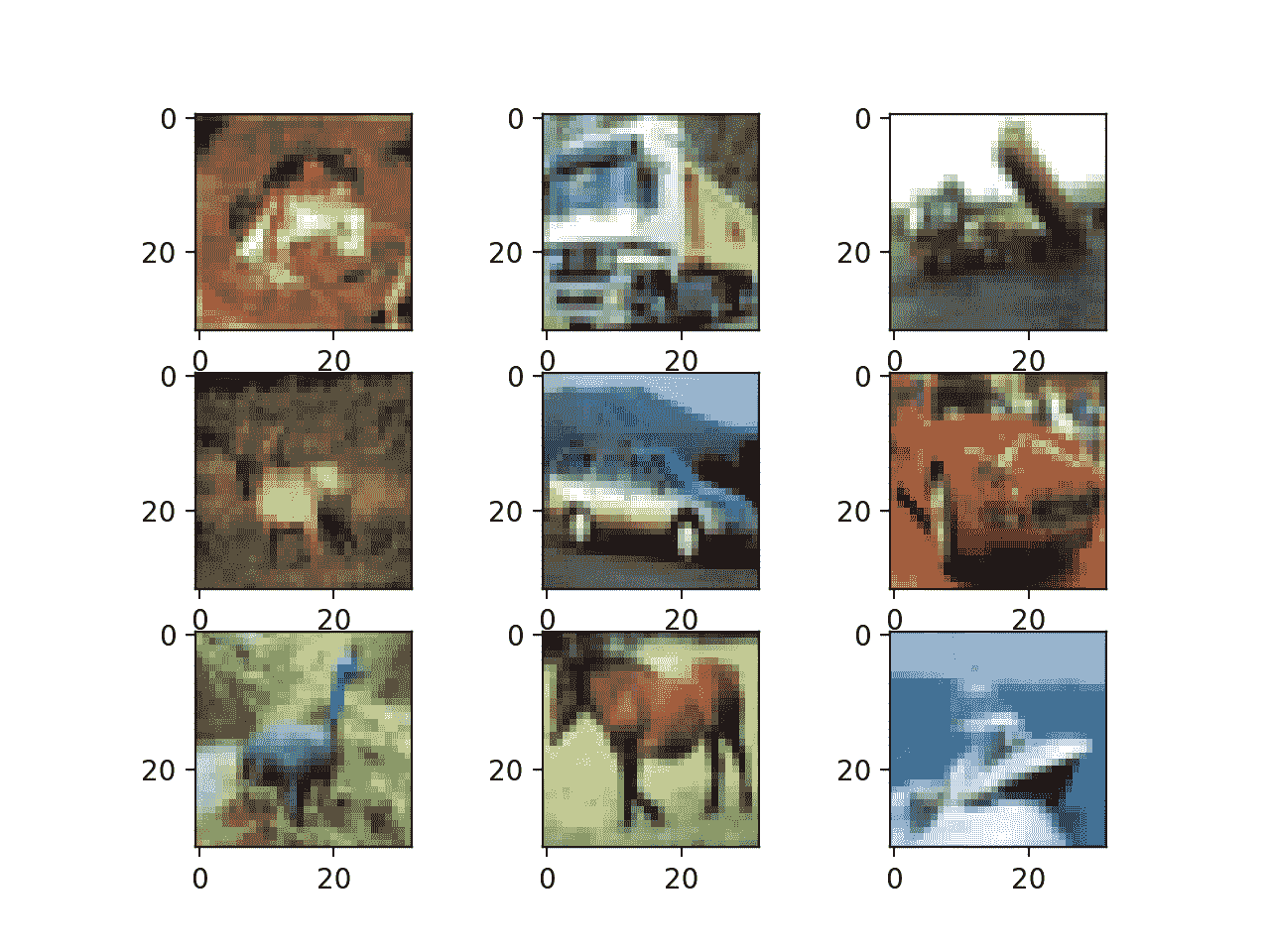
从 CIFAR-10 数据集绘制图像子集
模型评估测试线束
CIFAR-10 数据集可以成为开发和实践使用卷积神经网络解决图像分类问题的方法的有用起点。
我们可以从零开始开发一个新的模型,而不是回顾数据集上表现良好的模型的文献。
数据集已经有了一个我们将使用的定义良好的训练和测试数据集。另一种方法是用 k=5 或 k=10 进行 k 倍交叉验证。如果有足够的资源,这是可取的。在这种情况下,为了确保本教程中的示例在合理的时间内执行,我们将不使用 k-fold 交叉验证。
测试线束的设计是模块化的,我们可以为每个部件开发单独的功能。如果我们愿意,这允许测试装具的给定方面与其余部分分开修改或互换。
我们可以用五个关键元素来开发这个测试工具。它们是数据集的加载、数据集的准备、模型的定义、模型的评估和结果的呈现。
加载数据集
我们知道一些关于数据集的事情。
例如,我们知道图像都是预分割的(例如,每个图像包含单个对象),图像都具有相同的 32×32 像素的正方形大小,并且图像是彩色的。因此,我们几乎可以立即加载图像并将其用于建模。
# load dataset
(trainX, trainY), (testX, testY) = cifar10.load_data()
我们还知道有 10 个类,类被表示为唯一的整数。
因此,我们可以对每个样本的类元素使用一热编码,将整数转换为 10 元素二进制向量,类值的索引为 1。我们可以通过*to _ classic()*效用函数来实现。
# one hot encode target values
trainY = to_categorical(trainY)
testY = to_categorical(testY)
load_dataset() 函数实现了这些行为,可以用来加载数据集。
# load train and test dataset
def load_dataset():
	# load dataset
	(trainX, trainY), (testX, testY) = cifar10.load_data()
	# one hot encode target values
	trainY = to_categorical(trainY)
	testY = to_categorical(testY)
	return trainX, trainY, testX, testY
准备像素数据
我们知道,数据集中每个图像的像素值都是无符号整数,范围在无颜色和全色之间,或者在 0 到 255 之间。
我们不知道缩放用于建模的像素值的最佳方式,但是我们知道需要一些缩放。
一个好的起点是归一化像素值,例如将它们重新缩放到范围[0,1]。这包括首先将数据类型从无符号整数转换为浮点数,然后将像素值除以最大值。
# convert from integers to floats
train_norm = train.astype('float32')
test_norm = test.astype('float32')
# normalize to range 0-1
train_norm = train_norm / 255.0
test_norm = test_norm / 255.0
下面的 prep_pixels() 函数实现了这些行为,并提供了需要缩放的训练和测试数据集的像素值。
# scale pixels
def prep_pixels(train, test):
	# convert from integers to floats
	train_norm = train.astype('float32')
	test_norm = test.astype('float32')
	# normalize to range 0-1
	train_norm = train_norm / 255.0
	test_norm = test_norm / 255.0
	# return normalized images
	return train_norm, test_norm
在任何建模之前,必须调用该函数来准备像素值。
定义模型
接下来,我们需要一种建立神经网络模型的方法。
下面的 define_model() 函数将定义并返回该模型,并且可以为我们希望稍后评估的给定模型配置进行填充或替换。
# define cnn model
def define_model():
	model = Sequential()
	# ...
	return model
评估模型
在模型定义之后,我们需要对其进行拟合和评估。
拟合模型需要指定训练时期的数量和批次大小。我们现在将使用通用的 100 个训练时期和 64 个适度的批量。
最好使用单独的验证数据集,例如通过将训练数据集分成训练集和验证集。在这种情况下,我们不会分割数据,而是使用测试数据集作为验证数据集,以保持示例简单。
测试数据集可以像验证数据集一样使用,并在每个训练周期结束时进行评估。这将在每个时期的训练和测试数据集上产生模型评估分数的轨迹,该轨迹可以在以后绘制。
# fit model
history = model.fit(trainX, trainY, epochs=100, batch_size=64, validation_data=(testX, testY), verbose=0)
一旦模型合适,我们就可以直接在测试数据集上对其进行评估。
# evaluate model
_, acc = model.evaluate(testX, testY, verbose=0)
呈现结果
一旦评估了模型,我们就可以展示结果了。
有两个关键方面需要介绍:训练期间模型学习行为的诊断和模型表现的估计。
首先,诊断包括创建一个线图,显示训练期间模型在列车和测试集上的表现。这些图对于了解模型是过拟合、欠拟合还是非常适合数据集很有价值。
我们将创建一个有两个支线剧情的单一人物,一个是损失,一个是准确性。蓝色线将指示训练数据集上的模型表现,橙色线将指示等待测试数据集上的表现。下面的*summary _ diagnostics()*函数在给定收集的训练历史的情况下创建并显示该图。剧情保存到文件中,特别是与脚本同名的文件,扩展名为“ png ”。
# plot diagnostic learning curves
def summarize_diagnostics(history):
	# plot loss
	pyplot.subplot(211)
	pyplot.title('Cross Entropy Loss')
	pyplot.plot(history.history['loss'], color='blue', label='train')
	pyplot.plot(history.history['val_loss'], color='orange', label='test')
	# plot accuracy
	pyplot.subplot(212)
	pyplot.title('Classification Accuracy')
	pyplot.plot(history.history['accuracy'], color='blue', label='train')
	pyplot.plot(history.history['val_accuracy'], color='orange', label='test')
	# save plot to file
	filename = sys.argv[0].split('/')[-1]
	pyplot.savefig(filename + '_plot.png')
	pyplot.close()
接下来,我们可以在测试数据集上报告最终的模型表现。
这可以通过直接打印分类准确率来实现。
print('> %.3f' % (acc * 100.0))
完整示例
我们需要一个驱动测试线束的功能。
这包括调用所有的定义函数。下面的*run _ test _ 线束()*函数实现了这一点,并且可以被调用来启动给定模型的评估。
# run the test harness for evaluating a model
def run_test_harness():
	# load dataset
	trainX, trainY, testX, testY = load_dataset()
	# prepare pixel data
	trainX, testX = prep_pixels(trainX, testX)
	# define model
	model = define_model()
	# fit model
	history = model.fit(trainX, trainY, epochs=100, batch_size=64, validation_data=(testX, testY), verbose=0)
	# evaluate model
	_, acc = model.evaluate(testX, testY, verbose=0)
	print('> %.3f' % (acc * 100.0))
	# learning curves
	summarize_diagnostics(history)
我们现在有了测试装具所需的一切。
下面列出了 CIFAR-10 数据集测试工具的完整代码示例。
# test harness for evaluating models on the cifar10 dataset
import sys
from matplotlib import pyplot
from keras.datasets import cifar10
from keras.utils import to_categorical
from keras.models import Sequential
from keras.layers import Conv2D
from keras.layers import MaxPooling2D
from keras.layers import Dense
from keras.layers import Flatten
from keras.optimizers import SGD

# load train and test dataset
def load_dataset():
	# load dataset
	(trainX, trainY), (testX, testY) = cifar10.load_data()
	# one hot encode target values
	trainY = to_categorical(trainY)
	testY = to_categorical(testY)
	return trainX, trainY, testX, testY

# scale pixels
def prep_pixels(train, test):
	# convert from integers to floats
	train_norm = train.astype('float32')
	test_norm = test.astype('float32')
	# normalize to range 0-1
	train_norm = train_norm / 255.0
	test_norm = test_norm / 255.0
	# return normalized images
	return train_norm, test_norm

# define cnn model
def define_model():
	model = Sequential()
	# ...
	return model

# plot diagnostic learning curves
def summarize_diagnostics(history):
	# plot loss
	pyplot.subplot(211)
	pyplot.title('Cross Entropy Loss')
	pyplot.plot(history.history['loss'], color='blue', label='train')
	pyplot.plot(history.history['val_loss'], color='orange', label='test')
	# plot accuracy
	pyplot.subplot(212)
	pyplot.title('Classification Accuracy')
	pyplot.plot(history.history['accuracy'], color='blue', label='train')
	pyplot.plot(history.history['val_accuracy'], color='orange', label='test')
	# save plot to file
	filename = sys.argv[0].split('/')[-1]
	pyplot.savefig(filename + '_plot.png')
	pyplot.close()

# run the test harness for evaluating a model
def run_test_harness():
	# load dataset
	trainX, trainY, testX, testY = load_dataset()
	# prepare pixel data
	trainX, testX = prep_pixels(trainX, testX)
	# define model
	model = define_model()
	# fit model
	history = model.fit(trainX, trainY, epochs=100, batch_size=64, validation_data=(testX, testY), verbose=0)
	# evaluate model
	_, acc = model.evaluate(testX, testY, verbose=0)
	print('> %.3f' % (acc * 100.0))
	# learning curves
	summarize_diagnostics(history)

# entry point, run the test harness
run_test_harness()
该测试工具可以评估我们可能希望在 CIFAR-10 数据集上评估的任何有线电视新闻网模型,并且可以在中央处理器或图形处理器上运行。
注:原样,没有定义模型,所以这个完整的例子无法运行。
接下来,让我们看看如何定义和评估基线模型。
如何开发基线模型
我们现在可以研究 CIFAR-10 数据集的基线模型。
基线模型将建立一个最低的模型表现,我们所有的其他模型都可以与之进行比较,以及一个我们可以用作研究和改进基础的模型架构。
一个很好的起点是 VGG 模型的一般架构原则。这些是一个很好的起点,因为它们在 ILSVRC 2014 竞赛中取得了顶级的表现,并且因为体系结构的模块化结构易于理解和实现。有关 VGG 模型的更多详细信息,请参见 2015 年的论文“用于大规模图像识别的超深度卷积网络”
该架构包括堆叠卷积层和 3×3 小滤波器,然后是最大池层。这些层一起形成一个块,并且这些块可以重复,其中每个块中的过滤器的数量随着网络的深度而增加,例如对于模型的前四个块为 32、64、128、256。卷积层上使用填充来确保输出特征映射的高度和宽度与输入匹配。
我们可以在 CIFAR-10 问题上探索这种体系结构,并将具有这种体系结构的模型与具有 1、2 和 3 个数据块的模型进行比较。
每层将使用 ReLU 激活功能和 he 权重初始化,这通常是最佳实践。例如,3 块 VGG 风格的架构可以在 Keras 中定义如下:
# example of a 3-block vgg style architecture
model = Sequential()
model.add(Conv2D(32, (3, 3), activation='relu', kernel_initializer='he_uniform', padding='same', input_shape=(32, 32, 3)))
model.add(Conv2D(32, (3, 3), activation='relu', kernel_initializer='he_uniform', padding='same'))
model.add(MaxPooling2D((2, 2)))
model.add(Conv2D(64, (3, 3), activation='relu', kernel_initializer='he_uniform', padding='same'))
model.add(Conv2D(64, (3, 3), activation='relu', kernel_initializer='he_uniform', padding='same'))
model.add(MaxPooling2D((2, 2)))
model.add(Conv2D(128, (3, 3), activation='relu', kernel_initializer='he_uniform', padding='same'))
model.add(Conv2D(128, (3, 3), activation='relu', kernel_initializer='he_uniform', padding='same'))
model.add(MaxPooling2D((2, 2)))
...
这定义了模型的特征检测器部分。这必须与模型的分类器部分相结合,分类器部分解释特征并预测给定照片属于哪个类别。
对于我们研究的每个模型,这都是固定的。首先,从模型的特征提取部分输出的特征图必须展平。然后,我们可以用一个或多个完全连接的层来解释它们,然后输出预测。对于 10 个类,输出层必须有 10 个节点,并使用 softmax 激活功能。
# example output part of the model
model.add(Flatten())
model.add(Dense(128, activation='relu', kernel_initializer='he_uniform'))
model.add(Dense(10, activation='softmax'))
...
模型将使用随机梯度下降进行优化。
我们将使用 0.001 的适度学习率和 0.9 的大动量,这两者都是很好的一般起点。该模型将优化多类分类所需的分类交叉熵损失函数,并将监控分类准确率。
# compile model
opt = SGD(lr=0.001, momentum=0.9)
model.compile(optimizer=opt, loss='categorical_crossentropy', metrics=['accuracy'])
我们现在有足够的元素来定义我们的 VGG 风格的基线模型。我们可以用 1、2 和 3 个 VGG 模块定义三种不同的模型架构,这要求我们定义 3 个不同版本的 define_model() 函数,如下所示。
要测试每个模型,必须使用上一节中定义的测试工具和下面定义的新版本的*定义 _ 模型()*功能创建新的脚本(例如 model_baseline1.py 、 model_baseline2.py 、…)。
让我们依次看一下每个 define_model() 函数以及对生成的测试线束的评估。
基线:1 个 VGG 区块
下面列出了一个 VGG 区块的 define_model() 功能。
# define cnn model
def define_model():
	model = Sequential()
	model.add(Conv2D(32, (3, 3), activation='relu', kernel_initializer='he_uniform', padding='same', input_shape=(32, 32, 3)))
	model.add(Conv2D(32, (3, 3), activation='relu', kernel_initializer='he_uniform', padding='same'))
	model.add(MaxPooling2D((2, 2)))
	model.add(Flatten())
	model.add(Dense(128, activation='relu', kernel_initializer='he_uniform'))
	model.add(Dense(10, activation='softmax'))
	# compile model
	opt = SGD(lr=0.001, momentum=0.9)
	model.compile(optimizer=opt, loss='categorical_crossentropy', metrics=['accuracy'])
	return model
在测试线束中运行模型首先会在测试数据集上打印分类准确率。
注:考虑到算法或评估程序的随机性,或数值准确率的差异,您的结果可能会有所不同。考虑运行该示例几次,并比较平均结果。
在这种情况下,我们可以看到该模型实现了不到 70%的分类准确率。
> 67.070
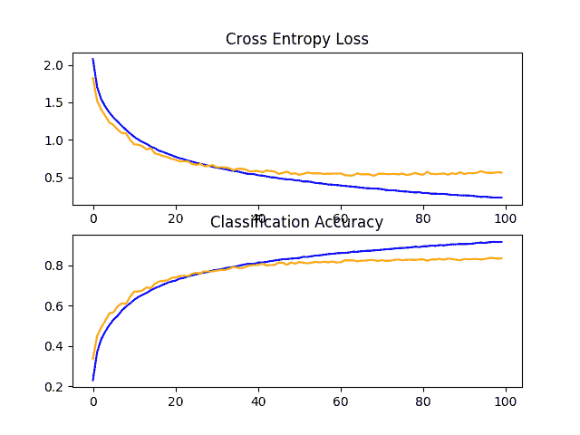
创建一个图形并保存到文件中,显示在训练和测试数据集上训练期间模型的学习曲线,包括损失和准确率。
在这种情况下,我们可以看到模型快速地覆盖了测试数据集。如果我们查看损失图(顶部图),我们可以看到模型在训练数据集(蓝色)上的表现继续提高,而在测试数据集(橙色)上的表现提高,然后在大约 15 个时期开始变差。
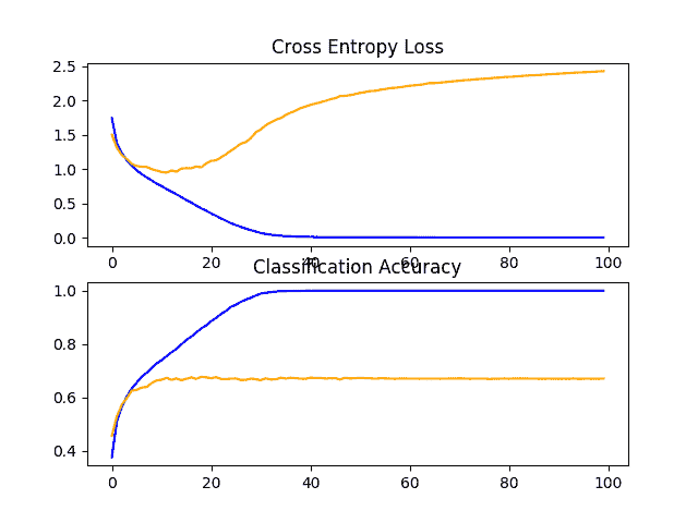
CIFAR-10 数据集上 VGG 1 基线的学习曲线线图
基线:2 个 VGG 区块
下面列出了两个 VGG 区块的 define_model() 函数。
# define cnn model
def define_model():
	model = Sequential()
	model.add(Conv2D(32, (3, 3), activation='relu', kernel_initializer='he_uniform', padding='same', input_shape=(32, 32, 3)))
	model.add(Conv2D(32, (3, 3), activation='relu', kernel_initializer='he_uniform', padding='same'))
	model.add(MaxPooling2D((2, 2)))
	model.add(Conv2D(64, (3, 3), activation='relu', kernel_initializer='he_uniform', padding='same'))
	model.add(Conv2D(64, (3, 3), activation='relu', kernel_initializer='he_uniform', padding='same'))
	model.add(MaxPooling2D((2, 2)))
	model.add(Flatten())
	model.add(Dense(128, activation='relu', kernel_initializer='he_uniform'))
	model.add(Dense(10, activation='softmax'))
	# compile model
	opt = SGD(lr=0.001, momentum=0.9)
	model.compile(optimizer=opt, loss='categorical_crossentropy', metrics=['accuracy'])
	return model
在测试线束中运行模型首先会在测试数据集上打印分类准确率。
注:考虑到算法或评估程序的随机性,或数值准确率的差异,您的结果可能会有所不同。考虑运行该示例几次,并比较平均结果。
在这种情况下,我们可以看到具有两个块的模型比具有单个块的模型表现更好:这是一个好迹象。
> 71.080
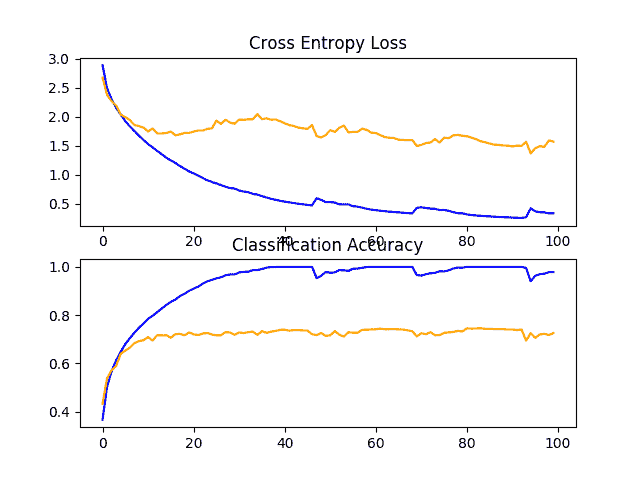
创建一个显示学习曲线的图形并保存到文件中。在这种情况下,我们继续看到强劲的过拟合。
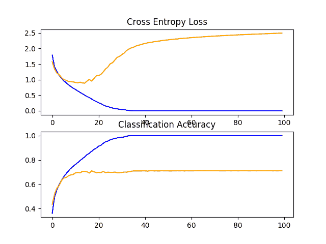
CIFAR-10 数据集上 VGG 2 基线的学习曲线线图
基线:3 个 VGG 区块
下面列出了三个 VGG 区块的 define_model() 功能。
# define cnn model
def define_model():
	model = Sequential()
	model.add(Conv2D(32, (3, 3), activation='relu', kernel_initializer='he_uniform', padding='same', input_shape=(32, 32, 3)))
	model.add(Conv2D(32, (3, 3), activation='relu', kernel_initializer='he_uniform', padding='same'))
	model.add(MaxPooling2D((2, 2)))
	model.add(Conv2D(64, (3, 3), activation='relu', kernel_initializer='he_uniform', padding='same'))
	model.add(Conv2D(64, (3, 3), activation='relu', kernel_initializer='he_uniform', padding='same'))
	model.add(MaxPooling2D((2, 2)))
	model.add(Conv2D(128, (3, 3), activation='relu', kernel_initializer='he_uniform', padding='same'))
	model.add(Conv2D(128, (3, 3), activation='relu', kernel_initializer='he_uniform', padding='same'))
	model.add(MaxPooling2D((2, 2)))
	model.add(Flatten())
	model.add(Dense(128, activation='relu', kernel_initializer='he_uniform'))
	model.add(Dense(10, activation='softmax'))
	# compile model
	opt = SGD(lr=0.001, momentum=0.9)
	model.compile(optimizer=opt, loss='categorical_crossentropy', metrics=['accuracy'])
	return model
在测试线束中运行模型首先会在测试数据集上打印分类准确率。
注:考虑到算法或评估程序的随机性,或数值准确率的差异,您的结果可能会有所不同。考虑运行该示例几次,并比较平均结果。
在这种情况下,随着模型深度的增加,表现又有了适度的提高。
> 73.500
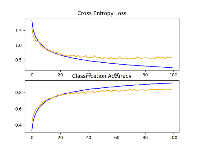
回顾显示学习曲线的数字,我们再次看到在最初的 20 个训练阶段中出现了戏剧性的过度适应。
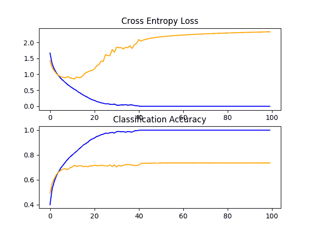
CIFAR-10 数据集上 VGG 3 基线的学习曲线线图
讨论
我们探索了基于 VGG 架构的三种不同模式。
结果可以总结如下,尽管我们必须假设这些结果中存在一些方差,因为算法具有随机性:
- VGG 1 : 67,070%
- vgg 2:71 080%
- VGG 3 : 73,500%
在所有情况下,模型都能够学习训练数据集,显示出对训练数据集的改进,至少持续到 40 个时代,也许更多。这是一个好的迹象,因为它表明这个问题是可以学习的,并且所有三个模型都有足够的能力来学习这个问题。
模型在测试数据集上的结果表明,随着模型深度的增加,分类准确率会提高。如果对四层和五层模型进行评估,这种趋势可能会继续下去,这可能是一个有趣的扩展。尽管如此,这三个模型在大约 15 到 20 个时期都显示出同样的戏剧性过拟合模式。
这些结果表明,具有三个 VGG 区块的模型是我们研究的良好起点或基线模型。
结果还表明,该模型需要正则化来解决测试数据集的快速过拟合。更一般地,结果表明,研究减缓模型收敛(学习率)的技术可能是有用的。这可能包括一些技术,如数据扩充、学习率计划、批量变化等等。
在下一节中,我们将研究一些提高模型表现的想法。
如何开发改进的模型
现在我们已经建立了一个基线模型,即具有三个模块的 VGG 体系结构,我们可以研究模型和训练算法的修改,以提高表现。
我们将首先关注两个主要领域来解决观察到的严重过拟合,即正则化和数据扩充。
正则化技术
我们可以尝试许多正则化技术,尽管观察到的过拟合的性质表明,也许提前停止是不合适的,并且减慢收敛速度的技术可能是有用的。
我们将研究丢失和权重正则化或权重衰减的影响。
丢弃正规化
丢弃是一种简单的技术,它会将节点随机地从网络中丢弃。它有一个规则化的效果,因为剩余的节点必须适应拾起被移除的节点的松弛。
有关丢弃的更多信息,请参阅帖子:
可以通过添加新的 drop 层将 drop 添加到模型中,其中移除的节点数量被指定为参数。将 drop 添加到模型中有许多模式,比如在模型中的什么位置添加层以及使用多少 drop。
在这种情况下,我们将在每个最大池层之后和完全连接层之后添加丢弃层,并使用 20%的固定丢弃率(例如,保留 80%的节点)。
下面列出了更新后的 VGG 3 基线丢弃模型。
# define cnn model
def define_model():
	model = Sequential()
	model.add(Conv2D(32, (3, 3), activation='relu', kernel_initializer='he_uniform', padding='same', input_shape=(32, 32, 3)))
	model.add(Conv2D(32, (3, 3), activation='relu', kernel_initializer='he_uniform', padding='same'))
	model.add(MaxPooling2D((2, 2)))
	model.add(Dropout(0.2))
	model.add(Conv2D(64, (3, 3), activation='relu', kernel_initializer='he_uniform', padding='same'))
	model.add(Conv2D(64, (3, 3), activation='relu', kernel_initializer='he_uniform', padding='same'))
	model.add(MaxPooling2D((2, 2)))
	model.add(Dropout(0.2))
	model.add(Conv2D(128, (3, 3), activation='relu', kernel_initializer='he_uniform', padding='same'))
	model.add(Conv2D(128, (3, 3), activation='relu', kernel_initializer='he_uniform', padding='same'))
	model.add(MaxPooling2D((2, 2)))
	model.add(Dropout(0.2))
	model.add(Flatten())
	model.add(Dense(128, activation='relu', kernel_initializer='he_uniform'))
	model.add(Dropout(0.2))
	model.add(Dense(10, activation='softmax'))
	# compile model
	opt = SGD(lr=0.001, momentum=0.9)
	model.compile(optimizer=opt, loss='categorical_crossentropy', metrics=['accuracy'])
	return model
为了完整起见,下面提供了完整的代码列表。
# baseline model with dropout on the cifar10 dataset
import sys
from matplotlib import pyplot
from keras.datasets import cifar10
from keras.utils import to_categorical
from keras.models import Sequential
from keras.layers import Conv2D
from keras.layers import MaxPooling2D
from keras.layers import Dense
from keras.layers import Flatten
from keras.layers import Dropout
from keras.optimizers import SGD

# load train and test dataset
def load_dataset():
	# load dataset
	(trainX, trainY), (testX, testY) = cifar10.load_data()
	# one hot encode target values
	trainY = to_categorical(trainY)
	testY = to_categorical(testY)
	return trainX, trainY, testX, testY

# scale pixels
def prep_pixels(train, test):
	# convert from integers to floats
	train_norm = train.astype('float32')
	test_norm = test.astype('float32')
	# normalize to range 0-1
	train_norm = train_norm / 255.0
	test_norm = test_norm / 255.0
	# return normalized images
	return train_norm, test_norm

# define cnn model
def define_model():
	model = Sequential()
	model.add(Conv2D(32, (3, 3), activation='relu', kernel_initializer='he_uniform', padding='same', input_shape=(32, 32, 3)))
	model.add(Conv2D(32, (3, 3), activation='relu', kernel_initializer='he_uniform', padding='same'))
	model.add(MaxPooling2D((2, 2)))
	model.add(Dropout(0.2))
	model.add(Conv2D(64, (3, 3), activation='relu', kernel_initializer='he_uniform', padding='same'))
	model.add(Conv2D(64, (3, 3), activation='relu', kernel_initializer='he_uniform', padding='same'))
	model.add(MaxPooling2D((2, 2)))
	model.add(Dropout(0.2))
	model.add(Conv2D(128, (3, 3), activation='relu', kernel_initializer='he_uniform', padding='same'))
	model.add(Conv2D(128, (3, 3), activation='relu', kernel_initializer='he_uniform', padding='same'))
	model.add(MaxPooling2D((2, 2)))
	model.add(Dropout(0.2))
	model.add(Flatten())
	model.add(Dense(128, activation='relu', kernel_initializer='he_uniform'))
	model.add(Dropout(0.2))
	model.add(Dense(10, activation='softmax'))
	# compile model
	opt = SGD(lr=0.001, momentum=0.9)
	model.compile(optimizer=opt, loss='categorical_crossentropy', metrics=['accuracy'])
	return model

# plot diagnostic learning curves
def summarize_diagnostics(history):
	# plot loss
	pyplot.subplot(211)
	pyplot.title('Cross Entropy Loss')
	pyplot.plot(history.history['loss'], color='blue', label='train')
	pyplot.plot(history.history['val_loss'], color='orange', label='test')
	# plot accuracy
	pyplot.subplot(212)
	pyplot.title('Classification Accuracy')
	pyplot.plot(history.history['accuracy'], color='blue', label='train')
	pyplot.plot(history.history['val_accuracy'], color='orange', label='test')
	# save plot to file
	filename = sys.argv[0].split('/')[-1]
	pyplot.savefig(filename + '_plot.png')
	pyplot.close()

# run the test harness for evaluating a model
def run_test_harness():
	# load dataset
	trainX, trainY, testX, testY = load_dataset()
	# prepare pixel data
	trainX, testX = prep_pixels(trainX, testX)
	# define model
	model = define_model()
	# fit model
	history = model.fit(trainX, trainY, epochs=100, batch_size=64, validation_data=(testX, testY), verbose=0)
	# evaluate model
	_, acc = model.evaluate(testX, testY, verbose=0)
	print('> %.3f' % (acc * 100.0))
	# learning curves
	summarize_diagnostics(history)

# entry point, run the test harness
run_test_harness()
在测试线束中运行模型会在测试数据集上打印分类准确率。
注:考虑到算法或评估程序的随机性,或数值准确率的差异,您的结果可能会有所不同。考虑运行该示例几次,并比较平均结果。
在这种情况下,我们可以看到分类准确率提高了约 10%,从没有丢弃的约 73%提高到丢弃的约 83%。
> 83.450
回顾模型的学习曲线,我们可以看到过拟合已经得到解决。该模型在大约 40 或 50 个时期内收敛良好,此时测试数据集没有进一步的改进。
这是一个伟大的结果。我们可以详细说明这个模型,并以大约 10 个时期的耐心添加早期停止,以便在训练期间在测试集上保存一个表现良好的模型,此时没有观察到进一步的改进。
我们也可以尝试探索一种学习率计划,在测试集停滞后降低学习率。
丢弃率表现不错,我们不知道 20%的选择率是最好的。我们可以探索其他丢弃率,以及丢弃层在模型架构中的不同定位。
CIFAR-10 数据集上缺失基线模型的学习曲线线图
重量衰减
权重正则化或权重衰减涉及更新损失函数,以与模型权重的大小成比例地惩罚模型。
这具有正则化效果,因为较大的权重导致更复杂和不太稳定的模型,而较小的权重通常更稳定和更通用。
要了解有关权重正则化的更多信息,请查看帖子:
我们可以通过定义“核 _ 正则化器”参数并指定正则化类型,为卷积层和全连通层添加权重正则化。在这种情况下,我们将使用 L2 权重正则化,用于神经网络的最常见类型和 0.001 的合理默认权重。
下面列出了带有重量衰减的更新基线模型。
# define cnn model
def define_model():
	model = Sequential()
	model.add(Conv2D(32, (3, 3), activation='relu', kernel_initializer='he_uniform', padding='same', kernel_regularizer=l2(0.001), input_shape=(32, 32, 3)))
	model.add(Conv2D(32, (3, 3), activation='relu', kernel_initializer='he_uniform', padding='same', kernel_regularizer=l2(0.001)))
	model.add(MaxPooling2D((2, 2)))
	model.add(Conv2D(64, (3, 3), activation='relu', kernel_initializer='he_uniform', padding='same', kernel_regularizer=l2(0.001)))
	model.add(Conv2D(64, (3, 3), activation='relu', kernel_initializer='he_uniform', padding='same', kernel_regularizer=l2(0.001)))
	model.add(MaxPooling2D((2, 2)))
	model.add(Conv2D(128, (3, 3), activation='relu', kernel_initializer='he_uniform', padding='same', kernel_regularizer=l2(0.001)))
	model.add(Conv2D(128, (3, 3), activation='relu', kernel_initializer='he_uniform', padding='same', kernel_regularizer=l2(0.001)))
	model.add(MaxPooling2D((2, 2)))
	model.add(Flatten())
	model.add(Dense(128, activation='relu', kernel_initializer='he_uniform', kernel_regularizer=l2(0.001)))
	model.add(Dense(10, activation='softmax'))
	# compile model
	opt = SGD(lr=0.001, momentum=0.9)
	model.compile(optimizer=opt, loss='categorical_crossentropy', metrics=['accuracy'])
	return model
为了完整起见,下面提供了完整的代码列表。
# baseline model with weight decay on the cifar10 dataset
import sys
from matplotlib import pyplot
from keras.datasets import cifar10
from keras.utils import to_categorical
from keras.models import Sequential
from keras.layers import Conv2D
from keras.layers import MaxPooling2D
from keras.layers import Dense
from keras.layers import Flatten
from keras.optimizers import SGD
from keras.regularizers import l2

# load train and test dataset
def load_dataset():
	# load dataset
	(trainX, trainY), (testX, testY) = cifar10.load_data()
	# one hot encode target values
	trainY = to_categorical(trainY)
	testY = to_categorical(testY)
	return trainX, trainY, testX, testY

# scale pixels
def prep_pixels(train, test):
	# convert from integers to floats
	train_norm = train.astype('float32')
	test_norm = test.astype('float32')
	# normalize to range 0-1
	train_norm = train_norm / 255.0
	test_norm = test_norm / 255.0
	# return normalized images
	return train_norm, test_norm

# define cnn model
def define_model():
	model = Sequential()
	model.add(Conv2D(32, (3, 3), activation='relu', kernel_initializer='he_uniform', padding='same', kernel_regularizer=l2(0.001), input_shape=(32, 32, 3)))
	model.add(Conv2D(32, (3, 3), activation='relu', kernel_initializer='he_uniform', padding='same', kernel_regularizer=l2(0.001)))
	model.add(MaxPooling2D((2, 2)))
	model.add(Conv2D(64, (3, 3), activation='relu', kernel_initializer='he_uniform', padding='same', kernel_regularizer=l2(0.001)))
	model.add(Conv2D(64, (3, 3), activation='relu', kernel_initializer='he_uniform', padding='same', kernel_regularizer=l2(0.001)))
	model.add(MaxPooling2D((2, 2)))
	model.add(Conv2D(128, (3, 3), activation='relu', kernel_initializer='he_uniform', padding='same', kernel_regularizer=l2(0.001)))
	model.add(Conv2D(128, (3, 3), activation='relu', kernel_initializer='he_uniform', padding='same', kernel_regularizer=l2(0.001)))
	model.add(MaxPooling2D((2, 2)))
	model.add(Flatten())
	model.add(Dense(128, activation='relu', kernel_initializer='he_uniform', kernel_regularizer=l2(0.001)))
	model.add(Dense(10, activation='softmax'))
	# compile model
	opt = SGD(lr=0.001, momentum=0.9)
	model.compile(optimizer=opt, loss='categorical_crossentropy', metrics=['accuracy'])
	return model

# plot diagnostic learning curves
def summarize_diagnostics(history):
	# plot loss
	pyplot.subplot(211)
	pyplot.title('Cross Entropy Loss')
	pyplot.plot(history.history['loss'], color='blue', label='train')
	pyplot.plot(history.history['val_loss'], color='orange', label='test')
	# plot accuracy
	pyplot.subplot(212)
	pyplot.title('Classification Accuracy')
	pyplot.plot(history.history['accuracy'], color='blue', label='train')
	pyplot.plot(history.history['val_accuracy'], color='orange', label='test')
	# save plot to file
	filename = sys.argv[0].split('/')[-1]
	pyplot.savefig(filename + '_plot.png')
	pyplot.close()

# run the test harness for evaluating a model
def run_test_harness():
	# load dataset
	trainX, trainY, testX, testY = load_dataset()
	# prepare pixel data
	trainX, testX = prep_pixels(trainX, testX)
	# define model
	model = define_model()
	# fit model
	history = model.fit(trainX, trainY, epochs=100, batch_size=64, validation_data=(testX, testY), verbose=0)
	# evaluate model
	_, acc = model.evaluate(testX, testY, verbose=0)
	print('> %.3f' % (acc * 100.0))
	# learning curves
	summarize_diagnostics(history)

# entry point, run the test harness
run_test_harness()
在测试线束中运行模型会打印测试数据集的分类准确率。
注:考虑到算法或评估程序的随机性,或数值准确率的差异,您的结果可能会有所不同。考虑运行该示例几次,并比较平均结果。
在这种情况下,我们在测试集上看不到模型表现的改善;事实上,我们看到分类准确率从大约 73%下降到大约 72%。
> 72.550
回顾学习曲线,我们确实看到过拟合略有减少,但影响不如丢弃有效。
我们或许可以通过使用更大的权重,比如 0.01 甚至 0.1,来改善权重衰减的效果。
CIFAR-10 数据集上权重衰减基线模型的学习曲线线图
日期增加
数据扩充包括用小的随机修改复制训练数据集中的例子。
这具有正则化效果,因为它既扩展了训练数据集,又允许模型学习相同的一般特征,尽管是以更一般化的方式。
有许多类型的数据扩充可以应用。假设数据集由对象的小照片组成,我们不希望使用过度偏斜图像的增强,以便可以保留和使用图像中的有用特征。
可能有用的随机增强类型包括水平翻转、图像的微小移动以及图像的小缩放或裁剪。
我们将研究简单增强对基线图像的影响,特别是水平翻转和图像高度和宽度 10%的移动。
这可以在 Keras 中使用 ImageDataGenerator 类实现;例如:
# create data generator
datagen = ImageDataGenerator(width_shift_range=0.1, height_shift_range=0.1, horizontal_flip=True)
# prepare iterator
it_train = datagen.flow(trainX, trainY, batch_size=64)
这可以在训练期间通过将迭代器传递给 model.fit_generator() 函数并定义单个时期内的批次数量来使用。
# fit model
steps = int(trainX.shape[0] / 64)
history = model.fit_generator(it_train, steps_per_epoch=steps, epochs=100, validation_data=(testX, testY), verbose=0)
不需要对模型进行更改。
支持数据扩充的*run _ test _ 线束()*功能的更新版本如下。
# run the test harness for evaluating a model
def run_test_harness():
	# load dataset
	trainX, trainY, testX, testY = load_dataset()
	# prepare pixel data
	trainX, testX = prep_pixels(trainX, testX)
	# define model
	model = define_model()
	# create data generator
	datagen = ImageDataGenerator(width_shift_range=0.1, height_shift_range=0.1, horizontal_flip=True)
	# prepare iterator
	it_train = datagen.flow(trainX, trainY, batch_size=64)
	# fit model
	steps = int(trainX.shape[0] / 64)
	history = model.fit_generator(it_train, steps_per_epoch=steps, epochs=100, validation_data=(testX, testY), verbose=0)
	# evaluate model
	_, acc = model.evaluate(testX, testY, verbose=0)
	print('> %.3f' % (acc * 100.0))
	# learning curves
	summarize_diagnostics(history)
为了完整起见,下面提供了完整的代码列表。
# baseline model with data augmentation on the cifar10 dataset
import sys
from matplotlib import pyplot
from keras.datasets import cifar10
from keras.utils import to_categorical
from keras.models import Sequential
from keras.layers import Conv2D
from keras.layers import MaxPooling2D
from keras.layers import Dense
from keras.layers import Flatten
from keras.optimizers import SGD
from keras.preprocessing.image import ImageDataGenerator

# load train and test dataset
def load_dataset():
	# load dataset
	(trainX, trainY), (testX, testY) = cifar10.load_data()
	# one hot encode target values
	trainY = to_categorical(trainY)
	testY = to_categorical(testY)
	return trainX, trainY, testX, testY

# scale pixels
def prep_pixels(train, test):
	# convert from integers to floats
	train_norm = train.astype('float32')
	test_norm = test.astype('float32')
	# normalize to range 0-1
	train_norm = train_norm / 255.0
	test_norm = test_norm / 255.0
	# return normalized images
	return train_norm, test_norm

# define cnn model
def define_model():
	model = Sequential()
	model.add(Conv2D(32, (3, 3), activation='relu', kernel_initializer='he_uniform', padding='same', input_shape=(32, 32, 3)))
	model.add(Conv2D(32, (3, 3), activation='relu', kernel_initializer='he_uniform', padding='same'))
	model.add(MaxPooling2D((2, 2)))
	model.add(Conv2D(64, (3, 3), activation='relu', kernel_initializer='he_uniform', padding='same'))
	model.add(Conv2D(64, (3, 3), activation='relu', kernel_initializer='he_uniform', padding='same'))
	model.add(MaxPooling2D((2, 2)))
	model.add(Conv2D(128, (3, 3), activation='relu', kernel_initializer='he_uniform', padding='same'))
	model.add(Conv2D(128, (3, 3), activation='relu', kernel_initializer='he_uniform', padding='same'))
	model.add(MaxPooling2D((2, 2)))
	model.add(Flatten())
	model.add(Dense(128, activation='relu', kernel_initializer='he_uniform'))
	model.add(Dense(10, activation='softmax'))
	# compile model
	opt = SGD(lr=0.001, momentum=0.9)
	model.compile(optimizer=opt, loss='categorical_crossentropy', metrics=['accuracy'])
	return model

# plot diagnostic learning curves
def summarize_diagnostics(history):
	# plot loss
	pyplot.subplot(211)
	pyplot.title('Cross Entropy Loss')
	pyplot.plot(history.history['loss'], color='blue', label='train')
	pyplot.plot(history.history['val_loss'], color='orange', label='test')
	# plot accuracy
	pyplot.subplot(212)
	pyplot.title('Classification Accuracy')
	pyplot.plot(history.history['accuracy'], color='blue', label='train')
	pyplot.plot(history.history['val_accuracy'], color='orange', label='test')
	# save plot to file
	filename = sys.argv[0].split('/')[-1]
	pyplot.savefig(filename + '_plot.png')
	pyplot.close()

# run the test harness for evaluating a model
def run_test_harness():
	# load dataset
	trainX, trainY, testX, testY = load_dataset()
	# prepare pixel data
	trainX, testX = prep_pixels(trainX, testX)
	# define model
	model = define_model()
	# create data generator
	datagen = ImageDataGenerator(width_shift_range=0.1, height_shift_range=0.1, horizontal_flip=True)
	# prepare iterator
	it_train = datagen.flow(trainX, trainY, batch_size=64)
	# fit model
	steps = int(trainX.shape[0] / 64)
	history = model.fit_generator(it_train, steps_per_epoch=steps, epochs=100, validation_data=(testX, testY), verbose=0)
	# evaluate model
	_, acc = model.evaluate(testX, testY, verbose=0)
	print('> %.3f' % (acc * 100.0))
	# learning curves
	summarize_diagnostics(history)

# entry point, run the test harness
run_test_harness()
在测试线束中运行模型会在测试数据集上打印分类准确率。
注:考虑到算法或评估程序的随机性,或数值准确率的差异,您的结果可能会有所不同。考虑运行该示例几次,并比较平均结果。
在这种情况下,我们看到了模型表现的另一个大的改进,很像我们看到的丢弃。在这种情况下,从基线模型的约 73%提高到约 84%,提高了约 11%。
> 84.470
回顾学习曲线,我们看到模型表现有类似于丢弃的改善,尽管损失图表明测试集上的模型表现可能比丢弃稍早停滞。
结果表明,同时使用丢失和数据增加的配置可能是有效的。
在 CIFAR-10 数据集上增加数据的基线模型的学习曲线的线图
讨论
在本节中,我们探索了三种旨在减缓模型收敛速度的方法。
结果摘要如下:
- 基线+丢弃率 : 83.450%
- 基线+权重衰减 : 72.550%
- 基线+数据增加 : 84.470%
结果表明,下降和数据增加都有预期的效果,而重量下降,至少对于所选的配置,没有。
现在模型学习得很好,我们可以寻找正在工作的改进,以及正在工作的组合。
如何进一步改进
在前面的部分中,我们发现,当丢失和数据增加被添加到基线模型中时,会产生一个很好地学习问题的模型。
我们现在将研究这些技术的改进,看看我们是否能进一步提高模型的表现。具体来说,我们将研究一个变体的丢弃正规化,并结合丢弃与数据增加。
学习已经变慢,因此我们将研究增加训练时期的数量,以便在需要时给模型足够的空间,从而在学习曲线中暴露学习动态。
脱落正则化的变分
丢弃是非常好的工作,所以它可能值得研究丢弃是如何应用于模型的变化。
一个有趣的变化是将丢弃率从 20%提高到 25%或 30%。另一个有趣的变化是,在模型的分类器部分,使用一种模式,在完全连接的层,从第一块的 20%,第二块的 30%,以此类推,到 50%。
这种随着模型深度的增加而减少的现象是常见的模式。这是有效的,因为它迫使模型深处的层比更接近输入的层更规则。
下面定义了根据模型深度增加丢弃率百分比的模式更新的丢弃基线模型。
# define cnn model
def define_model():
	model = Sequential()
	model.add(Conv2D(32, (3, 3), activation='relu', kernel_initializer='he_uniform', padding='same', input_shape=(32, 32, 3)))
	model.add(Conv2D(32, (3, 3), activation='relu', kernel_initializer='he_uniform', padding='same'))
	model.add(MaxPooling2D((2, 2)))
	model.add(Dropout(0.2))
	model.add(Conv2D(64, (3, 3), activation='relu', kernel_initializer='he_uniform', padding='same'))
	model.add(Conv2D(64, (3, 3), activation='relu', kernel_initializer='he_uniform', padding='same'))
	model.add(MaxPooling2D((2, 2)))
	model.add(Dropout(0.3))
	model.add(Conv2D(128, (3, 3), activation='relu', kernel_initializer='he_uniform', padding='same'))
	model.add(Conv2D(128, (3, 3), activation='relu', kernel_initializer='he_uniform', padding='same'))
	model.add(MaxPooling2D((2, 2)))
	model.add(Dropout(0.4))
	model.add(Flatten())
	model.add(Dense(128, activation='relu', kernel_initializer='he_uniform'))
	model.add(Dropout(0.5))
	model.add(Dense(10, activation='softmax'))
	# compile model
	opt = SGD(lr=0.001, momentum=0.9)
	model.compile(optimizer=opt, loss='categorical_crossentropy', metrics=['accuracy'])
	return model
为了完整起见,下面提供了包含此更改的完整代码列表。
# baseline model with increasing dropout on the cifar10 dataset
import sys
from matplotlib import pyplot
from keras.datasets import cifar10
from keras.utils import to_categorical
from keras.models import Sequential
from keras.layers import Conv2D
from keras.layers import MaxPooling2D
from keras.layers import Dense
from keras.layers import Flatten
from keras.layers import Dropout
from keras.optimizers import SGD

# load train and test dataset
def load_dataset():
	# load dataset
	(trainX, trainY), (testX, testY) = cifar10.load_data()
	# one hot encode target values
	trainY = to_categorical(trainY)
	testY = to_categorical(testY)
	return trainX, trainY, testX, testY

# scale pixels
def prep_pixels(train, test):
	# convert from integers to floats
	train_norm = train.astype('float32')
	test_norm = test.astype('float32')
	# normalize to range 0-1
	train_norm = train_norm / 255.0
	test_norm = test_norm / 255.0
	# return normalized images
	return train_norm, test_norm

# define cnn model
def define_model():
	model = Sequential()
	model.add(Conv2D(32, (3, 3), activation='relu', kernel_initializer='he_uniform', padding='same', input_shape=(32, 32, 3)))
	model.add(Conv2D(32, (3, 3), activation='relu', kernel_initializer='he_uniform', padding='same'))
	model.add(MaxPooling2D((2, 2)))
	model.add(Dropout(0.2))
	model.add(Conv2D(64, (3, 3), activation='relu', kernel_initializer='he_uniform', padding='same'))
	model.add(Conv2D(64, (3, 3), activation='relu', kernel_initializer='he_uniform', padding='same'))
	model.add(MaxPooling2D((2, 2)))
	model.add(Dropout(0.3))
	model.add(Conv2D(128, (3, 3), activation='relu', kernel_initializer='he_uniform', padding='same'))
	model.add(Conv2D(128, (3, 3), activation='relu', kernel_initializer='he_uniform', padding='same'))
	model.add(MaxPooling2D((2, 2)))
	model.add(Dropout(0.4))
	model.add(Flatten())
	model.add(Dense(128, activation='relu', kernel_initializer='he_uniform'))
	model.add(Dropout(0.5))
	model.add(Dense(10, activation='softmax'))
	# compile model
	opt = SGD(lr=0.001, momentum=0.9)
	model.compile(optimizer=opt, loss='categorical_crossentropy', metrics=['accuracy'])
	return model

# plot diagnostic learning curves
def summarize_diagnostics(history):
	# plot loss
	pyplot.subplot(211)
	pyplot.title('Cross Entropy Loss')
	pyplot.plot(history.history['loss'], color='blue', label='train')
	pyplot.plot(history.history['val_loss'], color='orange', label='test')
	# plot accuracy
	pyplot.subplot(212)
	pyplot.title('Classification Accuracy')
	pyplot.plot(history.history['accuracy'], color='blue', label='train')
	pyplot.plot(history.history['val_accuracy'], color='orange', label='test')
	# save plot to file
	filename = sys.argv[0].split('/')[-1]
	pyplot.savefig(filename + '_plot.png')
	pyplot.close()

# run the test harness for evaluating a model
def run_test_harness():
	# load dataset
	trainX, trainY, testX, testY = load_dataset()
	# prepare pixel data
	trainX, testX = prep_pixels(trainX, testX)
	# define model
	model = define_model()
	# fit model
	history = model.fit(trainX, trainY, epochs=200, batch_size=64, validation_data=(testX, testY), verbose=0)
	# evaluate model
	_, acc = model.evaluate(testX, testY, verbose=0)
	print('> %.3f' % (acc * 100.0))
	# learning curves
	summarize_diagnostics(history)

# entry point, run the test harness
run_test_harness()
在测试线束中运行模型会在测试数据集上打印分类准确率。
注:考虑到算法或评估程序的随机性,或数值准确率的差异,您的结果可能会有所不同。考虑运行该示例几次,并比较平均结果。
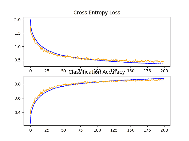
在这种情况下,我们可以看到从大约 83%的固定丢弃率到大约 84%的增加丢弃率的适度提升。
> 84.690
回顾学习曲线,我们可以看到模型收敛得很好,测试数据集上的表现可能停滞在大约 110 到 125 个时期。与固定丢弃率的学习曲线相比,我们可以再次看到,学习速度进一步放缓,允许在不过拟合的情况下进一步细化模型。
这是对该模型进行研究的一个富有成果的领域,也许更多的脱落层和/或更积极的脱落会导致进一步的改进。
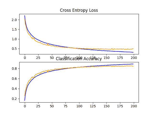
在 CIFAR-10 数据集上,基线模型的学习曲线随着缺失的增加而线性变化
丢弃和数据增加
在前一节中,我们发现丢失和数据增加都会导致模型表现的显著提高。
在本节中,我们可以尝试将这两种变化结合到模型中,看看是否可以实现进一步的改进。具体来说,两种正则化技术一起使用是否会比单独使用任何一种技术产生更好的表现。
为了完整起见,下面提供了具有固定丢失和数据增加的模型的完整代码列表。
# baseline model with dropout and data augmentation on the cifar10 dataset
import sys
from matplotlib import pyplot
from keras.datasets import cifar10
from keras.utils import to_categorical
from keras.models import Sequential
from keras.layers import Conv2D
from keras.layers import MaxPooling2D
from keras.layers import Dense
from keras.layers import Flatten
from keras.optimizers import SGD
from keras.preprocessing.image import ImageDataGenerator
from keras.layers import Dropout

# load train and test dataset
def load_dataset():
	# load dataset
	(trainX, trainY), (testX, testY) = cifar10.load_data()
	# one hot encode target values
	trainY = to_categorical(trainY)
	testY = to_categorical(testY)
	return trainX, trainY, testX, testY

# scale pixels
def prep_pixels(train, test):
	# convert from integers to floats
	train_norm = train.astype('float32')
	test_norm = test.astype('float32')
	# normalize to range 0-1
	train_norm = train_norm / 255.0
	test_norm = test_norm / 255.0
	# return normalized images
	return train_norm, test_norm

# define cnn model
def define_model():
	model = Sequential()
	model.add(Conv2D(32, (3, 3), activation='relu', kernel_initializer='he_uniform', padding='same', input_shape=(32, 32, 3)))
	model.add(Conv2D(32, (3, 3), activation='relu', kernel_initializer='he_uniform', padding='same'))
	model.add(MaxPooling2D((2, 2)))
	model.add(Dropout(0.2))
	model.add(Conv2D(64, (3, 3), activation='relu', kernel_initializer='he_uniform', padding='same'))
	model.add(Conv2D(64, (3, 3), activation='relu', kernel_initializer='he_uniform', padding='same'))
	model.add(MaxPooling2D((2, 2)))
	model.add(Dropout(0.2))
	model.add(Conv2D(128, (3, 3), activation='relu', kernel_initializer='he_uniform', padding='same'))
	model.add(Conv2D(128, (3, 3), activation='relu', kernel_initializer='he_uniform', padding='same'))
	model.add(MaxPooling2D((2, 2)))
	model.add(Dropout(0.2))
	model.add(Flatten())
	model.add(Dense(128, activation='relu', kernel_initializer='he_uniform'))
	model.add(Dropout(0.2))
	model.add(Dense(10, activation='softmax'))
	# compile model
	opt = SGD(lr=0.001, momentum=0.9)
	model.compile(optimizer=opt, loss='categorical_crossentropy', metrics=['accuracy'])
	return model

# plot diagnostic learning curves
def summarize_diagnostics(history):
	# plot loss
	pyplot.subplot(211)
	pyplot.title('Cross Entropy Loss')
	pyplot.plot(history.history['loss'], color='blue', label='train')
	pyplot.plot(history.history['val_loss'], color='orange', label='test')
	# plot accuracy
	pyplot.subplot(212)
	pyplot.title('Classification Accuracy')
	pyplot.plot(history.history['accuracy'], color='blue', label='train')
	pyplot.plot(history.history['val_accuracy'], color='orange', label='test')
	# save plot to file
	filename = sys.argv[0].split('/')[-1]
	pyplot.savefig(filename + '_plot.png')
	pyplot.close()

# run the test harness for evaluating a model
def run_test_harness():
	# load dataset
	trainX, trainY, testX, testY = load_dataset()
	# prepare pixel data
	trainX, testX = prep_pixels(trainX, testX)
	# define model
	model = define_model()
	# create data generator
	datagen = ImageDataGenerator(width_shift_range=0.1, height_shift_range=0.1, horizontal_flip=True)
	# prepare iterator
	it_train = datagen.flow(trainX, trainY, batch_size=64)
	# fit model
	steps = int(trainX.shape[0] / 64)
	history = model.fit_generator(it_train, steps_per_epoch=steps, epochs=200, validation_data=(testX, testY), verbose=0)
	# evaluate model
	_, acc = model.evaluate(testX, testY, verbose=0)
	print('> %.3f' % (acc * 100.0))
	# learning curves
	summarize_diagnostics(history)

# entry point, run the test harness
run_test_harness()
在测试线束中运行模型会在测试数据集上打印分类准确率。
注:考虑到算法或评估程序的随机性,或数值准确率的差异,您的结果可能会有所不同。考虑运行该示例几次,并比较平均结果。
在这种情况下,我们可以看到,正如我们所希望的那样,同时使用这两种正则化技术已经在测试集上进一步提升了模型表现。在这种情况下,将大约 83%的固定丢失率和大约 84%的数据增加率相结合,已经导致分类准确率提高到大约 85%。
> 85.880
回顾学习曲线,我们可以看到模型的收敛行为也优于单独的固定丢失和数据增加。在没有过度适应的情况下,学习速度有所减缓,允许持续改进。
情节还表明,学习可能没有停滞不前,如果允许继续,可能会继续提高,但可能非常温和。
如果在整个模型的深度范围内使用一种增加丢弃率的模式,而不是固定的丢弃率,结果可能会进一步改善。
在 CIFAR-10 数据集上具有缺失和数据增加的基线模型的学习曲线的线图
丢失和数据增加以及批量标准化
我们可以从几个方面来扩展前面的例子。
首先,我们可以将训练纪元的数量从 200 个增加到 400 个,给模型更多的改进机会。
接下来,我们可以添加批处理规范化,以努力稳定学习,并可能加快学习过程。为了抵消这种加速,我们可以通过将丢失从固定模式改为增加模式来增加正则化。
更新后的模型定义如下所示。
# define cnn model
def define_model():
	model = Sequential()
	model.add(Conv2D(32, (3, 3), activation='relu', kernel_initializer='he_uniform', padding='same', input_shape=(32, 32, 3)))
	model.add(BatchNormalization())
	model.add(Conv2D(32, (3, 3), activation='relu', kernel_initializer='he_uniform', padding='same'))
	model.add(BatchNormalization())
	model.add(MaxPooling2D((2, 2)))
	model.add(Dropout(0.2))
	model.add(Conv2D(64, (3, 3), activation='relu', kernel_initializer='he_uniform', padding='same'))
	model.add(BatchNormalization())
	model.add(Conv2D(64, (3, 3), activation='relu', kernel_initializer='he_uniform', padding='same'))
	model.add(BatchNormalization())
	model.add(MaxPooling2D((2, 2)))
	model.add(Dropout(0.3))
	model.add(Conv2D(128, (3, 3), activation='relu', kernel_initializer='he_uniform', padding='same'))
	model.add(BatchNormalization())
	model.add(Conv2D(128, (3, 3), activation='relu', kernel_initializer='he_uniform', padding='same'))
	model.add(BatchNormalization())
	model.add(MaxPooling2D((2, 2)))
	model.add(Dropout(0.4))
	model.add(Flatten())
	model.add(Dense(128, activation='relu', kernel_initializer='he_uniform'))
	model.add(BatchNormalization())
	model.add(Dropout(0.5))
	model.add(Dense(10, activation='softmax'))
	# compile model
	opt = SGD(lr=0.001, momentum=0.9)
	model.compile(optimizer=opt, loss='categorical_crossentropy', metrics=['accuracy'])
	return model
为了完整起见,下面提供了一个模型的完整代码列表,该模型具有越来越多的丢失、数据增加、批处理规范化和 400 个训练时期。
# baseline model with dropout and data augmentation on the cifar10 dataset
import sys
from matplotlib import pyplot
from keras.datasets import cifar10
from keras.utils import to_categorical
from keras.models import Sequential
from keras.layers import Conv2D
from keras.layers import MaxPooling2D
from keras.layers import Dense
from keras.layers import Flatten
from keras.optimizers import SGD
from keras.preprocessing.image import ImageDataGenerator
from keras.layers import Dropout
from keras.layers import BatchNormalization

# load train and test dataset
def load_dataset():
	# load dataset
	(trainX, trainY), (testX, testY) = cifar10.load_data()
	# one hot encode target values
	trainY = to_categorical(trainY)
	testY = to_categorical(testY)
	return trainX, trainY, testX, testY

# scale pixels
def prep_pixels(train, test):
	# convert from integers to floats
	train_norm = train.astype('float32')
	test_norm = test.astype('float32')
	# normalize to range 0-1
	train_norm = train_norm / 255.0
	test_norm = test_norm / 255.0
	# return normalized images
	return train_norm, test_norm

# define cnn model
def define_model():
	model = Sequential()
	model.add(Conv2D(32, (3, 3), activation='relu', kernel_initializer='he_uniform', padding='same', input_shape=(32, 32, 3)))
	model.add(BatchNormalization())
	model.add(Conv2D(32, (3, 3), activation='relu', kernel_initializer='he_uniform', padding='same'))
	model.add(BatchNormalization())
	model.add(MaxPooling2D((2, 2)))
	model.add(Dropout(0.2))
	model.add(Conv2D(64, (3, 3), activation='relu', kernel_initializer='he_uniform', padding='same'))
	model.add(BatchNormalization())
	model.add(Conv2D(64, (3, 3), activation='relu', kernel_initializer='he_uniform', padding='same'))
	model.add(BatchNormalization())
	model.add(MaxPooling2D((2, 2)))
	model.add(Dropout(0.3))
	model.add(Conv2D(128, (3, 3), activation='relu', kernel_initializer='he_uniform', padding='same'))
	model.add(BatchNormalization())
	model.add(Conv2D(128, (3, 3), activation='relu', kernel_initializer='he_uniform', padding='same'))
	model.add(BatchNormalization())
	model.add(MaxPooling2D((2, 2)))
	model.add(Dropout(0.4))
	model.add(Flatten())
	model.add(Dense(128, activation='relu', kernel_initializer='he_uniform'))
	model.add(BatchNormalization())
	model.add(Dropout(0.5))
	model.add(Dense(10, activation='softmax'))
	# compile model
	opt = SGD(lr=0.001, momentum=0.9)
	model.compile(optimizer=opt, loss='categorical_crossentropy', metrics=['accuracy'])
	return model

# plot diagnostic learning curves
def summarize_diagnostics(history):
	# plot loss
	pyplot.subplot(211)
	pyplot.title('Cross Entropy Loss')
	pyplot.plot(history.history['loss'], color='blue', label='train')
	pyplot.plot(history.history['val_loss'], color='orange', label='test')
	# plot accuracy
	pyplot.subplot(212)
	pyplot.title('Classification Accuracy')
	pyplot.plot(history.history['accuracy'], color='blue', label='train')
	pyplot.plot(history.history['val_accuracy'], color='orange', label='test')
	# save plot to file
	filename = sys.argv[0].split('/')[-1]
	pyplot.savefig(filename + '_plot.png')
	pyplot.close()

# run the test harness for evaluating a model
def run_test_harness():
	# load dataset
	trainX, trainY, testX, testY = load_dataset()
	# prepare pixel data
	trainX, testX = prep_pixels(trainX, testX)
	# define model
	model = define_model()
	# create data generator
	datagen = ImageDataGenerator(width_shift_range=0.1, height_shift_range=0.1, horizontal_flip=True)
	# prepare iterator
	it_train = datagen.flow(trainX, trainY, batch_size=64)
	# fit model
	steps = int(trainX.shape[0] / 64)
	history = model.fit_generator(it_train, steps_per_epoch=steps, epochs=400, validation_data=(testX, testY), verbose=0)
	# evaluate model
	_, acc = model.evaluate(testX, testY, verbose=0)
	print('> %.3f' % (acc * 100.0))
	# learning curves
	summarize_diagnostics(history)

# entry point, run the test harness
run_test_harness()
在测试线束中运行模型会在测试数据集上打印分类准确率。
注:考虑到算法或评估程序的随机性,或数值准确率的差异,您的结果可能会有所不同。考虑运行该示例几次,并比较平均结果。
在这种情况下,我们可以看到,我们实现了模型表现的进一步提升,达到约 88%的准确率,仅在丢失和数据增加方面就提高了约 84%,仅在丢失增加方面就提高了约 85%。
> 88.620
回顾学习曲线,我们可以看到模型的训练显示在近 400 个时期的持续改进。我们可以看到在大约 300 个时代,测试数据集可能会略有下降,但改善趋势确实会继续。
该模型可能受益于进一步的培训时代。
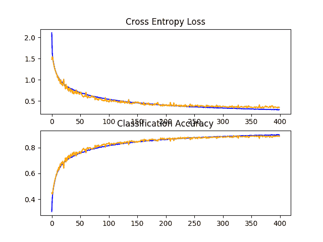
在 CIFAR-10 数据集上具有增加的缺失、数据增加和批量标准化的基线模型的学习曲线的线图
讨论
在本节中,我们探索了两种方法,这两种方法旨在扩展我们已知已经导致改进的模型变更
结果摘要如下:
- 基线+增加丢弃率 : 84.690%
- 基线+丢失+数据增加 : 85.880%
- 基线+增加丢失+数据增加+批量归一化 : 88.620%
模型现在学习得很好,我们可以很好地控制学习速度,而不会过拟合。
我们也许能够通过额外的正则化实现进一步的改进。这可以通过在后面的层中更积极地退出来实现。进一步增加重量衰减可能会改进模型。
到目前为止,我们还没有调整学习算法的超参数,例如学习率,这可能是最重要的超参数。我们可以期待随着学习率的适应性变化而进一步改进,例如使用适应性学习率技术,如 Adam 。一旦收敛,这些类型的变化可能有助于改进模型。
如何最终确定模型并做出预测
只要我们有想法,有时间和资源来测试,模型改进的过程可能会持续很长时间。
在某些时候,必须选择并采用最终的模型配置。在这种情况下,我们将保持简单,并使用基线模型(VGG 有 3 个区块)作为最终模型。
首先,我们将通过在整个训练数据集上拟合模型并将模型保存到文件中以备后用来最终确定我们的模型。然后,我们将加载模型,并在等待测试数据集上评估其表现,以了解所选模型在实践中的实际表现。最后,我们将使用保存的模型对单个图像进行预测。
保存最终模型
最终模型通常适合所有可用数据,例如所有训练和测试数据集的组合。
在本教程中,我们将仅在训练数据集上演示最终的模型拟合,以保持示例的简单性。
第一步是在整个训练数据集上拟合最终模型。
# fit model
model.fit(trainX, trainY, epochs=100, batch_size=64, verbose=0)
一旦合适,我们可以通过调用模型上的 save() 函数将最终模型保存到一个 H5 文件中,并传入选择的文件名。
# save model
model.save('final_model.h5')
注意:保存和加载 Keras 模型需要在您的工作站上安装 h5py 库。
下面列出了在训练数据集上拟合最终模型并将其保存到文件中的完整示例。
# save the final model to file
from keras.datasets import cifar10
from keras.utils import to_categorical
from keras.models import Sequential
from keras.layers import Conv2D
from keras.layers import MaxPooling2D
from keras.layers import Dense
from keras.layers import Flatten
from keras.optimizers import SGD

# load train and test dataset
def load_dataset():
	# load dataset
	(trainX, trainY), (testX, testY) = cifar10.load_data()
	# one hot encode target values
	trainY = to_categorical(trainY)
	testY = to_categorical(testY)
	return trainX, trainY, testX, testY

# scale pixels
def prep_pixels(train, test):
	# convert from integers to floats
	train_norm = train.astype('float32')
	test_norm = test.astype('float32')
	# normalize to range 0-1
	train_norm = train_norm / 255.0
	test_norm = test_norm / 255.0
	# return normalized images
	return train_norm, test_norm

# define cnn model
def define_model():
	model = Sequential()
	model.add(Conv2D(32, (3, 3), activation='relu', kernel_initializer='he_uniform', padding='same', input_shape=(32, 32, 3)))
	model.add(Conv2D(32, (3, 3), activation='relu', kernel_initializer='he_uniform', padding='same'))
	model.add(MaxPooling2D((2, 2)))
	model.add(Conv2D(64, (3, 3), activation='relu', kernel_initializer='he_uniform', padding='same'))
	model.add(Conv2D(64, (3, 3), activation='relu', kernel_initializer='he_uniform', padding='same'))
	model.add(MaxPooling2D((2, 2)))
	model.add(Conv2D(128, (3, 3), activation='relu', kernel_initializer='he_uniform', padding='same'))
	model.add(Conv2D(128, (3, 3), activation='relu', kernel_initializer='he_uniform', padding='same'))
	model.add(MaxPooling2D((2, 2)))
	model.add(Flatten())
	model.add(Dense(128, activation='relu', kernel_initializer='he_uniform'))
	model.add(Dense(10, activation='softmax'))
	# compile model
	opt = SGD(lr=0.001, momentum=0.9)
	model.compile(optimizer=opt, loss='categorical_crossentropy', metrics=['accuracy'])
	return model

# run the test harness for evaluating a model
def run_test_harness():
	# load dataset
	trainX, trainY, testX, testY = load_dataset()
	# prepare pixel data
	trainX, testX = prep_pixels(trainX, testX)
	# define model
	model = define_model()
	# fit model
	model.fit(trainX, trainY, epochs=100, batch_size=64, verbose=0)
	# save model
	model.save('final_model.h5')

# entry point, run the test harness
run_test_harness()
运行此示例后,您的当前工作目录中将有一个名为“ final_model.h5 ”的 4.3 兆字节文件。
评估最终模型
我们现在可以加载最终模型,并在等待测试数据集上对其进行评估。
如果我们有兴趣向项目涉众展示所选模型的表现,这是我们可以做的事情。
测试数据集用于评估和选择候选模型。因此,它不会成为一个好的最终测试支持数据集。然而,在这种情况下,我们将使用它作为一个保持数据集。
可通过 load_model() 功能加载模型。
下面列出了加载保存的模型并在测试数据集上对其进行评估的完整示例。
# evaluate the deep model on the test dataset
from keras.datasets import cifar10
from keras.models import load_model
from keras.utils import to_categorical

# load train and test dataset
def load_dataset():
	# load dataset
	(trainX, trainY), (testX, testY) = cifar10.load_data()
	# one hot encode target values
	trainY = to_categorical(trainY)
	testY = to_categorical(testY)
	return trainX, trainY, testX, testY

# scale pixels
def prep_pixels(train, test):
	# convert from integers to floats
	train_norm = train.astype('float32')
	test_norm = test.astype('float32')
	# normalize to range 0-1
	train_norm = train_norm / 255.0
	test_norm = test_norm / 255.0
	# return normalized images
	return train_norm, test_norm

# run the test harness for evaluating a model
def run_test_harness():
	# load dataset
	trainX, trainY, testX, testY = load_dataset()
	# prepare pixel data
	trainX, testX = prep_pixels(trainX, testX)
	# load model
	model = load_model('final_model.h5')
	# evaluate model on test dataset
	_, acc = model.evaluate(testX, testY, verbose=0)
	print('> %.3f' % (acc * 100.0))

# entry point, run the test harness
run_test_harness()
运行该示例将加载保存的模型,并在暂挂测试数据集上评估该模型。
计算并打印测试数据集中模型的分类准确率。
注:考虑到算法或评估程序的随机性,或数值准确率的差异,您的结果可能会有所不同。考虑运行该示例几次,并比较平均结果。
在这种情况下,我们可以看到模型达到了大约 73%的准确率,非常接近我们在评估模型作为测试工具的一部分时看到的准确率。
73.750
作出预测
我们可以使用保存的模型对新图像进行预测。
该模型假设新图像是彩色的,它们已经被分割,使得一幅图像包含一个居中的对象,并且图像的大小是 32×32 像素的正方形。
下面是从 CIFAR-10 测试数据集提取的图像。您可以将其保存在当前工作目录中,文件名为“ sample_image.png ”。
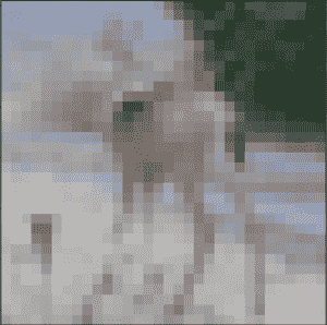
鹿
我们将假装这是一个全新的、看不见的图像,按照要求的方式准备,看看我们如何使用保存的模型来预测图像所代表的整数。
对于这个例子,我们期望类“ 4 ”为“鹿”。
首先,我们可以加载图像,并强制其大小为 32×32 像素。然后,可以调整加载图像的大小,使其具有单个通道,并表示数据集中的单个样本。 load_image() 函数实现了这一点,并将返回已加载的准备分类的图像。
重要的是,像素值的准备方式与在拟合最终模型时为训练数据集准备像素值的方式相同,在这种情况下,最终模型是归一化的。
# load and prepare the image
def load_image(filename):
	# load the image
	img = load_img(filename, target_size=(32, 32))
	# convert to array
	img = img_to_array(img)
	# reshape into a single sample with 3 channels
	img = img.reshape(1, 32, 32, 3)
	# prepare pixel data
	img = img.astype('float32')
	img = img / 255.0
	return img
接下来,我们可以像上一节一样加载模型,并调用*predict _ class()*函数来预测图像中的对象。
# predict the class
result = model.predict_classes(img)
下面列出了完整的示例。
# make a prediction for a new image.
from keras.preprocessing.image import load_img
from keras.preprocessing.image import img_to_array
from keras.models import load_model

# load and prepare the image
def load_image(filename):
	# load the image
	img = load_img(filename, target_size=(32, 32))
	# convert to array
	img = img_to_array(img)
	# reshape into a single sample with 3 channels
	img = img.reshape(1, 32, 32, 3)
	# prepare pixel data
	img = img.astype('float32')
	img = img / 255.0
	return img

# load an image and predict the class
def run_example():
	# load the image
	img = load_image('sample_image.png')
	# load model
	model = load_model('final_model.h5')
	# predict the class
	result = model.predict_classes(img)
	print(result[0])

# entry point, run the example
run_example()
运行该示例首先加载和准备图像,加载模型,然后正确预测加载的图像代表“鹿或类“ 4 ”。
4
扩展ˌ扩张
本节列出了一些您可能希望探索的扩展教程的想法。
- 像素缩放。探索缩放像素的替代技术,如居中和标准化,并比较表现。
- 学习率。探索替代学习率、自适应学习率和学习率计划,并比较绩效。
- 迁移学习。探索使用迁移学习,例如在此数据集上预先训练的 VGG-16 模型。
如果你探索这些扩展,我很想知道。
在下面的评论中发表你的发现。
进一步阅读
如果您想更深入地了解这个主题,本节将提供更多资源。
邮件
应用程序接口
文章
- 类别数据集结果,这个图像的类别是什么?
- CIFAR-10,维基百科。
- CIFAR-10 数据集和 CIFAR-100 数据集。
- CIFAR-10–图像中的对象识别,卡格尔。
- 简单 CNN 90%+,Pasquale Giovenale,Kaggle 。
摘要
在本教程中,您发现了如何从零开始为对象照片分类开发卷积神经网络模型。
具体来说,您了解到:
- 如何开发一个测试工具来开发一个健壮的模型评估,并为分类任务建立一个表现基线。
- 如何探索基线模型的扩展,以提高学习和模型能力。
- 如何开发最终模型,评估最终模型的表现,并使用它对新图像进行预测。
你有什么问题吗?
在下面的评论中提问,我会尽力回答。
用于 Fashion-MNIST 服装分类的深度学习 CNN
最后更新于 2020 年 8 月 28 日
时装-MNIST 服装分类问题是一个用于计算机视觉和深度学习的新标准数据集。
虽然数据集相对简单,但它可以作为学习和实践如何从零开始开发、评估和使用深度卷积神经网络进行图像分类的基础。这包括如何开发一个健壮的测试工具来评估模型的表现,如何探索模型的改进,以及如何保存模型并在以后加载它来对新数据进行预测。
在本教程中,您将发现如何从零开始开发用于服装分类的卷积神经网络。
完成本教程后,您将知道:
- 如何开发一个测试工具来开发一个健壮的模型评估,并为分类任务建立一个表现基线。
- 如何探索基线模型的扩展,以提高学习和模型能力。
- 如何开发最终模型,评估最终模型的表现,并使用它对新图像进行预测。
用我的新书计算机视觉深度学习启动你的项目,包括分步教程和所有示例的 Python 源代码文件。
我们开始吧。
- 更新 2019 年 6 月:修复了在 CV 循环之外定义模型的小错误。更新结果(感谢 Aditya)。
- 2019 年 10 月更新:针对 Keras 2.3 和 TensorFlow 2.0 更新。

如何从零开始为时尚 MNIST 服装分类开发深度卷积神经网络
图片由 Zdrovit Skurcz 提供,版权所有。
教程概述
本教程分为五个部分;它们是:
- 时尚 MNIST 服装分类
- 模型评估方法
- 如何开发基线模型
- 如何开发改进的模型
- 如何最终确定模型并做出预测
时尚 MNIST 服装分类
时尚-MNIST 数据集被提议作为 MNIST 数据集的更具挑战性的替代数据集。
它是一个数据集,由 60,000 个 28×28 像素的小正方形灰度图像组成,包括 10 种服装,如鞋子、t 恤、连衣裙等。下面列出了所有 0-9 整数到类标签的映射。
- 0: T 恤/上衣
- 1:裤子
- 2:套头衫
- 3:着装
- 4:外套
- 5:凉鞋
- 6:衬衫
- 7:运动鞋
- 8:包
- 9:踝靴
这是一个比 MNIST 更具挑战性的分类问题,通过深度学习卷积神经网络可以获得最佳结果,在等待测试数据集上的分类准确率约为 90%至 95%。
以下示例使用 Keras API 加载时尚 MNIST 数据集,并创建训练数据集中前九幅图像的图。
# example of loading the fashion mnist dataset
from matplotlib import pyplot
from keras.datasets import fashion_mnist
# load dataset
(trainX, trainy), (testX, testy) = fashion_mnist.load_data()
# summarize loaded dataset
print('Train: X=%s, y=%s' % (trainX.shape, trainy.shape))
print('Test: X=%s, y=%s' % (testX.shape, testy.shape))
# plot first few images
for i in range(9):
	# define subplot
	pyplot.subplot(330 + 1 + i)
	# plot raw pixel data
	pyplot.imshow(trainX[i], cmap=pyplot.get_cmap('gray'))
# show the figure
pyplot.show()
运行该示例将加载时尚 MNIST 训练和测试数据集,并打印它们的形状。
我们可以看到训练数据集中有 6 万个例子,测试数据集中有 1 万个例子,图像确实是 28×28 像素的正方形。
Train: X=(60000, 28, 28), y=(60000,)
Test: X=(10000, 28, 28), y=(10000,)
还创建了数据集中前九幅图像的图,显示这些图像确实是衣物的灰度照片。
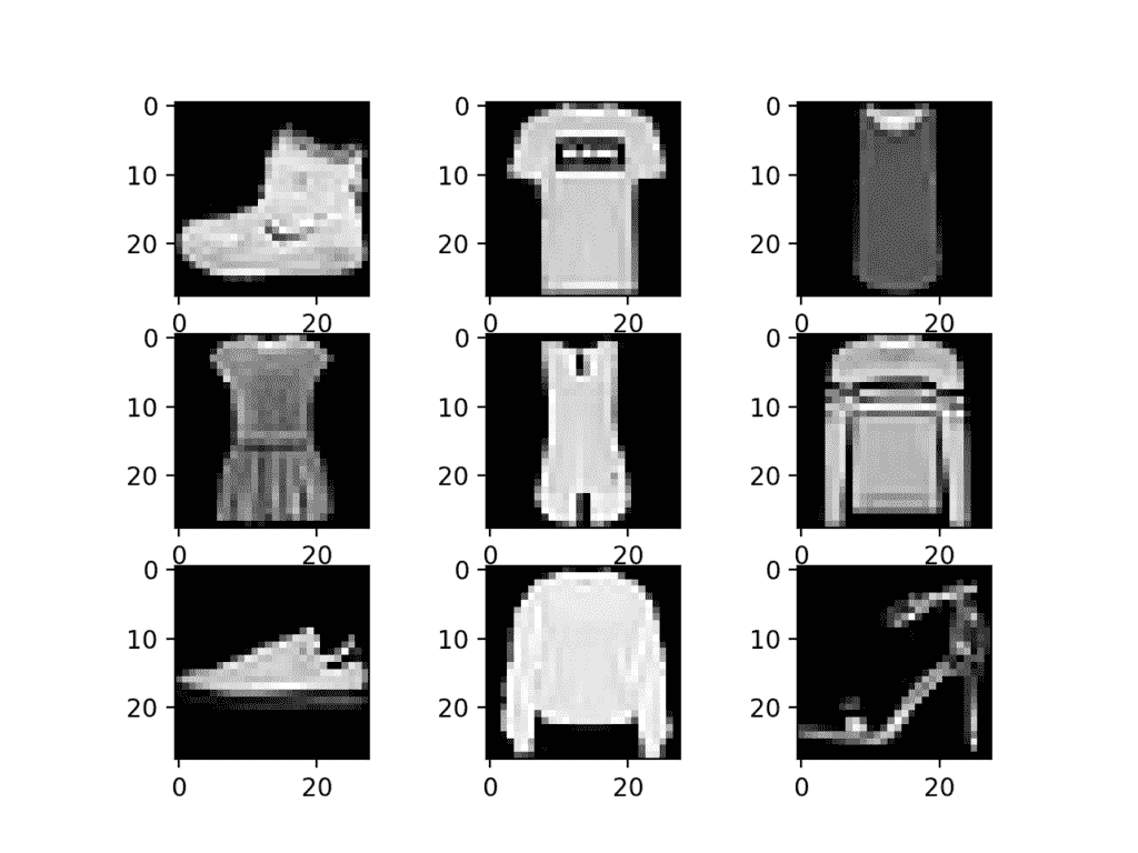
时尚 MNIST 数据集图像子集的绘图
模型评估方法
时尚 MNIST 数据集是作为对广泛使用的 MNIST 数据集的响应而开发的,由于使用了现代卷积神经网络,已经有效地解决了。
时尚-MNIST 被提议作为 MNIST 的替代品,尽管这个问题还没有解决,但通常有可能达到 10%或更低的错误率。像 MNIST 一样,它可以成为开发和实践使用卷积神经网络解决图像分类方法的有用起点。
我们可以从零开始开发一个新的模型,而不是回顾数据集上表现良好的模型的文献。
数据集已经有了我们可以使用的定义良好的训练和测试数据集。
为了估计给定训练运行的模型表现,我们可以进一步将训练集拆分为训练和验证数据集。然后,可以绘制每次运行的训练和验证数据集的表现,以提供学习曲线和对模型学习问题的深入了解。
Keras API 通过在训练模型时为 model.fit() 函数指定“ validation_data ”参数来支持这一点,该函数将返回一个对象,该对象描述所选损失的模型表现和每个训练时期的度量。
# record model performance on a validation dataset during training
history = model.fit(..., validation_data=(valX, valY))
为了估计模型在一般问题上的表现,我们可以使用 k 倍交叉验证,也许是 5 倍交叉验证。这将给出关于训练和测试数据集的差异以及学习算法的随机性质的模型方差的一些说明。模型的表现可以作为 k 倍的平均表现,用标准偏差给出,如果需要,可以用来估计置信区间。
我们可以使用 Sklearn API 中的 KFold 类来实现给定神经网络模型的 K 折交叉验证评估。有许多方法可以实现这一点,尽管我们可以选择一种灵活的方法,其中 KFold 仅用于指定用于每个拆分的行索引。
# example of k-fold cv for a neural net
data = ...
# prepare cross validation
kfold = KFold(5, shuffle=True, random_state=1)
# enumerate splits
for train_ix, test_ix in kfold.split(data):
        model = ...
	...
我们将保留实际的测试数据集,并将其用作最终模型的评估。
如何开发基线模型
第一步是开发一个基线模型。
这一点至关重要,因为它既涉及到为测试工具开发基础设施,以便我们设计的任何模型都可以在数据集上进行评估,又建立了问题模型表现的基线,通过该基线可以比较所有的改进。
测试线束的设计是模块化的,我们可以为每个部件开发单独的功能。如果我们愿意的话,这允许测试装具的给定方面独立于其他方面进行修改或交互改变。
我们可以用五个关键元素来开发这个测试工具。它们是数据集的加载、数据集的准备、模型的定义、模型的评估和结果的呈现。
加载数据集
我们知道一些关于数据集的事情。
例如,我们知道图像都是预分割的(例如,每个图像包含一件衣服),图像都具有相同的 28×28 像素的正方形大小,并且图像是灰度的。因此,我们可以加载图像并重塑数据阵列,使其具有单一颜色通道。
# load dataset
(trainX, trainY), (testX, testY) = fashion_mnist.load_data()
# reshape dataset to have a single channel
trainX = trainX.reshape((trainX.shape[0], 28, 28, 1))
testX = testX.reshape((testX.shape[0], 28, 28, 1))
我们还知道有 10 个类,类被表示为唯一的整数。
因此,我们可以对每个样本的类元素使用一热编码,将整数转换为 10 元素二进制向量,类值的索引为 1。我们可以通过*to _ classic()*效用函数来实现。
# one hot encode target values
trainY = to_categorical(trainY)
testY = to_categorical(testY)
load_dataset() 函数实现了这些行为,可以用来加载数据集。
# load train and test dataset
def load_dataset():
	# load dataset
	(trainX, trainY), (testX, testY) = fashion_mnist.load_data()
	# reshape dataset to have a single channel
	trainX = trainX.reshape((trainX.shape[0], 28, 28, 1))
	testX = testX.reshape((testX.shape[0], 28, 28, 1))
	# one hot encode target values
	trainY = to_categorical(trainY)
	testY = to_categorical(testY)
	return trainX, trainY, testX, testY
准备像素数据
我们知道,数据集中每个图像的像素值都是介于黑白或 0 到 255 之间的无符号整数。
我们不知道缩放用于建模的像素值的最佳方式,但是我们知道需要一些缩放。
一个好的起点是归一化灰度图像的像素值,例如将它们重新缩放到范围[0,1]。这包括首先将数据类型从无符号整数转换为浮点数,然后将像素值除以最大值。
# convert from integers to floats
train_norm = train.astype('float32')
test_norm = test.astype('float32')
# normalize to range 0-1
train_norm = train_norm / 255.0
test_norm = test_norm / 255.0
下面的 prep_pixels() 函数实现了这些行为,并提供了需要缩放的训练和测试数据集的像素值。
# scale pixels
def prep_pixels(train, test):
	# convert from integers to floats
	train_norm = train.astype('float32')
	test_norm = test.astype('float32')
	# normalize to range 0-1
	train_norm = train_norm / 255.0
	test_norm = test_norm / 255.0
	# return normalized images
	return train_norm, test_norm
在任何建模之前,必须调用该函数来准备像素值。
定义模型
接下来,我们需要为这个问题定义一个基线卷积神经网络模型。
该模型有两个主要方面:由卷积层和池化层组成的特征提取前端,以及进行预测的分类器后端。
对于卷积前端,我们可以从单个卷积层开始,它具有小的滤波器大小(3,3)和适度数量的滤波器(32),然后是最大池层。过滤图然后可以被展平以向分类器提供特征。
假设问题是一个多类分类,我们知道我们将需要一个具有 10 个节点的输出层,以便预测属于 10 个类中每一个的图像的概率分布。这也需要使用 softmax 激活功能。在特征提取器和输出层之间,我们可以添加一个密集层来解释特征,在本例中有 100 个节点。
所有层将使用 ReLU 激活功能和 he 权重初始化方案,两者都是最佳实践。
对于学习率为 0.01、动量为 0.9 的随机梯度下降优化器,我们将使用保守配置。分类交叉熵损失函数将被优化,适用于多类分类,我们将监控分类准确率度量,这是合适的,因为我们在 10 类中的每一类都有相同数量的例子。
下面的 define_model() 函数将定义并返回这个模型。
# define cnn model
def define_model():
	model = Sequential()
	model.add(Conv2D(32, (3, 3), activation='relu', kernel_initializer='he_uniform', input_shape=(28, 28, 1)))
	model.add(MaxPooling2D((2, 2)))
	model.add(Flatten())
	model.add(Dense(100, activation='relu', kernel_initializer='he_uniform'))
	model.add(Dense(10, activation='softmax'))
	# compile model
	opt = SGD(lr=0.01, momentum=0.9)
	model.compile(optimizer=opt, loss='categorical_crossentropy', metrics=['accuracy'])
	return model
评估模型
模型定义后,我们需要对其进行评估。
该模型将使用 5 重交叉验证进行评估。选择 k=5 的值是为了提供重复评估的基线,并且不要太大而需要很长的运行时间。每个测试集将占训练数据集的 20%,或者大约 12,000 个例子,接近于这个问题的实际测试集的大小。
训练数据集在被分割之前被混洗,并且每次都执行样本混洗,以便我们评估的任何模型在每个文件夹中都将具有相同的训练和测试数据集,从而提供苹果对苹果的比较。
我们将为一个适度的 10 个训练时期训练基线模型,默认批量为 32 个例子。每个折叠的测试集将用于在训练运行的每个时期评估模型,因此我们可以稍后创建学习曲线,并在运行结束时评估模型的表现。因此,我们将跟踪每次运行的结果历史,以及折叠的分类准确率。
下面的 evaluate_model() 函数实现了这些行为,将训练数据集作为参数,并返回一个准确性分数和训练历史的列表,稍后可以对其进行总结。
# evaluate a model using k-fold cross-validation
def evaluate_model(dataX, dataY, n_folds=5):
	scores, histories = list(), list()
	# prepare cross validation
	kfold = KFold(n_folds, shuffle=True, random_state=1)
	# enumerate splits
	for train_ix, test_ix in kfold.split(dataX):
		# define model
		model = define_model()
		# select rows for train and test
		trainX, trainY, testX, testY = dataX[train_ix], dataY[train_ix], dataX[test_ix], dataY[test_ix]
		# fit model
		history = model.fit(trainX, trainY, epochs=10, batch_size=32, validation_data=(testX, testY), verbose=0)
		# evaluate model
		_, acc = model.evaluate(testX, testY, verbose=0)
		print('> %.3f' % (acc * 100.0))
		# append scores
		scores.append(acc)
		histories.append(history)
	return scores, histories
呈现结果
一旦评估了模型,我们就可以展示结果了。
有两个关键方面需要介绍:训练期间模型学习行为的诊断和模型表现的估计。这些可以使用单独的函数来实现。
首先,诊断包括创建一个线图,显示在 k 折叠交叉验证的每个折叠期间,模型在列车和测试集上的表现。这些图对于了解模型是过拟合、欠拟合还是非常适合数据集很有价值。
我们将创建一个有两个支线剧情的单一人物,一个是损失,一个是准确性。蓝色线将指示训练数据集上的模型表现,橙色线将指示等待测试数据集上的表现。下面的*summary _ diagnostics()*函数在给定收集的训练历史的情况下创建并显示该图。
# plot diagnostic learning curves
def summarize_diagnostics(histories):
	for i in range(len(histories)):
		# plot loss
		pyplot.subplot(211)
		pyplot.title('Cross Entropy Loss')
		pyplot.plot(histories[i].history['loss'], color='blue', label='train')
		pyplot.plot(histories[i].history['val_loss'], color='orange', label='test')
		# plot accuracy
		pyplot.subplot(212)
		pyplot.title('Classification Accuracy')
		pyplot.plot(histories[i].history['accuracy'], color='blue', label='train')
		pyplot.plot(histories[i].history['val_accuracy'], color='orange', label='test')
	pyplot.show()
接下来,可以通过计算平均值和标准偏差来总结每次折叠期间收集的分类准确度分数。这提供了在该数据集上训练的模型的平均预期表现的估计,以及平均值的平均方差的估计。我们还将通过创建和显示一个方框和触须图来总结分数的分布。
下面的*summary _ performance()*函数为模型评估期间收集的给定分数列表实现了这一点。
# summarize model performance
def summarize_performance(scores):
	# print summary
	print('Accuracy: mean=%.3f std=%.3f, n=%d' % (mean(scores)*100, std(scores)*100, len(scores)))
	# box and whisker plots of results
	pyplot.boxplot(scores)
	pyplot.show()
完整示例
我们需要一个驱动测试线束的功能。
这包括调用所有的定义函数。
# run the test harness for evaluating a model
def run_test_harness():
	# load dataset
	trainX, trainY, testX, testY = load_dataset()
	# prepare pixel data
	trainX, testX = prep_pixels(trainX, testX)
	# evaluate model
	scores, histories = evaluate_model(trainX, trainY)
	# learning curves
	summarize_diagnostics(histories)
	# summarize estimated performance
	summarize_performance(scores)
我们现在拥有我们需要的一切;下面列出了 MNIST 数据集上基线卷积神经网络模型的完整代码示例。
# baseline cnn model for fashion mnist
from numpy import mean
from numpy import std
from matplotlib import pyplot
from sklearn.model_selection import KFold
from keras.datasets import fashion_mnist
from keras.utils import to_categorical
from keras.models import Sequential
from keras.layers import Conv2D
from keras.layers import MaxPooling2D
from keras.layers import Dense
from keras.layers import Flatten
from keras.optimizers import SGD

# load train and test dataset
def load_dataset():
	# load dataset
	(trainX, trainY), (testX, testY) = fashion_mnist.load_data()
	# reshape dataset to have a single channel
	trainX = trainX.reshape((trainX.shape[0], 28, 28, 1))
	testX = testX.reshape((testX.shape[0], 28, 28, 1))
	# one hot encode target values
	trainY = to_categorical(trainY)
	testY = to_categorical(testY)
	return trainX, trainY, testX, testY

# scale pixels
def prep_pixels(train, test):
	# convert from integers to floats
	train_norm = train.astype('float32')
	test_norm = test.astype('float32')
	# normalize to range 0-1
	train_norm = train_norm / 255.0
	test_norm = test_norm / 255.0
	# return normalized images
	return train_norm, test_norm

# define cnn model
def define_model():
	model = Sequential()
	model.add(Conv2D(32, (3, 3), activation='relu', kernel_initializer='he_uniform', input_shape=(28, 28, 1)))
	model.add(MaxPooling2D((2, 2)))
	model.add(Flatten())
	model.add(Dense(100, activation='relu', kernel_initializer='he_uniform'))
	model.add(Dense(10, activation='softmax'))
	# compile model
	opt = SGD(lr=0.01, momentum=0.9)
	model.compile(optimizer=opt, loss='categorical_crossentropy', metrics=['accuracy'])
	return model

# evaluate a model using k-fold cross-validation
def evaluate_model(dataX, dataY, n_folds=5):
	scores, histories = list(), list()
	# prepare cross validation
	kfold = KFold(n_folds, shuffle=True, random_state=1)
	# enumerate splits
	for train_ix, test_ix in kfold.split(dataX):
		# define model
		model = define_model()
		# select rows for train and test
		trainX, trainY, testX, testY = dataX[train_ix], dataY[train_ix], dataX[test_ix], dataY[test_ix]
		# fit model
		history = model.fit(trainX, trainY, epochs=10, batch_size=32, validation_data=(testX, testY), verbose=0)
		# evaluate model
		_, acc = model.evaluate(testX, testY, verbose=0)
		print('> %.3f' % (acc * 100.0))
		# append scores
		scores.append(acc)
		histories.append(history)
	return scores, histories

# plot diagnostic learning curves
def summarize_diagnostics(histories):
	for i in range(len(histories)):
		# plot loss
		pyplot.subplot(211)
		pyplot.title('Cross Entropy Loss')
		pyplot.plot(histories[i].history['loss'], color='blue', label='train')
		pyplot.plot(histories[i].history['val_loss'], color='orange', label='test')
		# plot accuracy
		pyplot.subplot(212)
		pyplot.title('Classification Accuracy')
		pyplot.plot(histories[i].history['accuracy'], color='blue', label='train')
		pyplot.plot(histories[i].history['val_accuracy'], color='orange', label='test')
	pyplot.show()

# summarize model performance
def summarize_performance(scores):
	# print summary
	print('Accuracy: mean=%.3f std=%.3f, n=%d' % (mean(scores)*100, std(scores)*100, len(scores)))
	# box and whisker plots of results
	pyplot.boxplot(scores)
	pyplot.show()

# run the test harness for evaluating a model
def run_test_harness():
	# load dataset
	trainX, trainY, testX, testY = load_dataset()
	# prepare pixel data
	trainX, testX = prep_pixels(trainX, testX)
	# evaluate model
	scores, histories = evaluate_model(trainX, trainY)
	# learning curves
	summarize_diagnostics(histories)
	# summarize estimated performance
	summarize_performance(scores)

# entry point, run the test harness
run_test_harness()
运行该示例会打印交叉验证过程中每个折叠的分类准确率。这有助于了解模型评估正在进行。
注:考虑到算法或评估程序的随机性,或数值准确率的差异,您的结果可能会有所不同。考虑运行该示例几次,并比较平均结果。
我们可以看到,对于每个折叠,基线模型实现了低于 10%的错误率,并且在两种情况下实现了 98%和 99%的准确性。这些都是好结果。
> 91.200
> 91.217
> 90.958
> 91.242
> 91.317
接下来,显示了一个诊断图,提供了对模型在每个折叠中的学习行为的洞察。
在这种情况下,我们可以看到该模型通常实现了良好的拟合,训练和测试学习曲线收敛。可能有一些轻微过拟合的迹象。
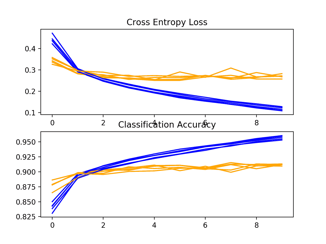
损失和准确性-学习-基线曲线-时尚模型-MNIST-数据集-k 倍期间-交叉验证
接下来,计算模型表现的总结。我们可以看到,在这种情况下,模型的估计技能约为 96%,这令人印象深刻。
Accuracy: mean=91.187 std=0.121, n=5
最后,创建一个方框和触须图来总结准确度分数的分布。
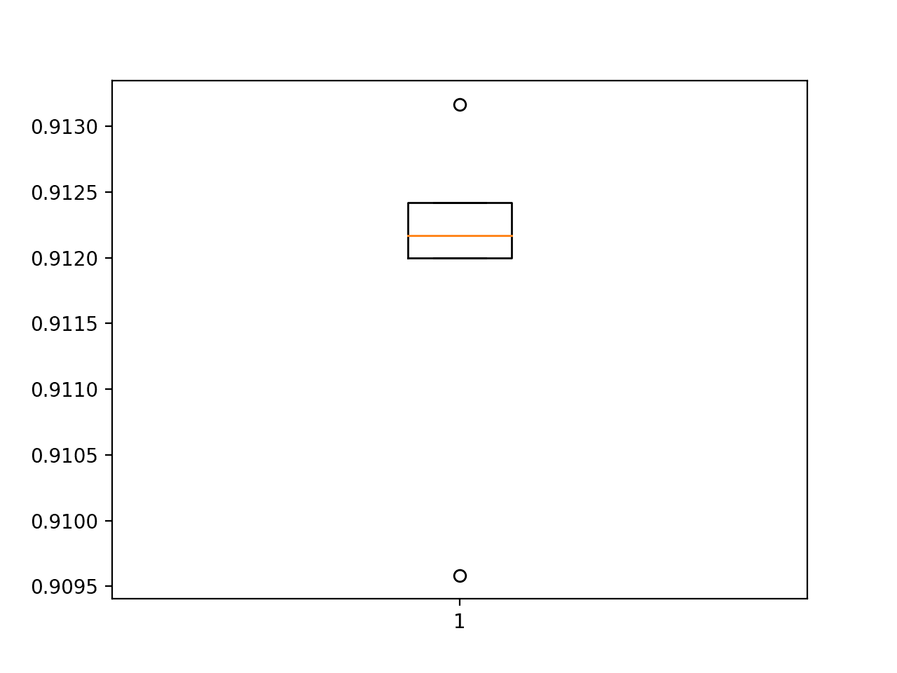
盒子-触须-准确度图-时尚基线模型分数-MNIST-数据集-评估-使用-k-折叠-交叉验证
正如我们所料,这种分布遍及 90 年代末。
我们现在有了一个健壮的测试工具和一个表现良好的基线模型。
如何开发改进的模型
我们有很多方法可以探索基线模型的改进。
我们将关注那些通常会带来改善的领域,即所谓的低挂水果。第一种是对卷积运算的改变,增加填充,第二种是在此基础上增加滤波器的数量。
填充卷积
向卷积运算添加填充通常可以导致更好的模型表现,因为更多的特征图输入图像被给予参与或贡献输出的机会
默认情况下,卷积运算使用“有效的”填充,这意味着卷积仅在可能的情况下应用。这可以更改为“相同的”填充,以便在输入周围添加零值,从而使输出具有与输入相同的大小。
...
model.add(Conv2D(32, (3, 3), padding='same', activation='relu', kernel_initializer='he_uniform', input_shape=(28, 28, 1)))
为了完整起见,下面提供了完整的代码列表,包括对填充的更改。
# model with padded convolutions for the fashion mnist dataset
from numpy import mean
from numpy import std
from matplotlib import pyplot
from sklearn.model_selection import KFold
from keras.datasets import fashion_mnist
from keras.utils import to_categorical
from keras.models import Sequential
from keras.layers import Conv2D
from keras.layers import MaxPooling2D
from keras.layers import Dense
from keras.layers import Flatten
from keras.optimizers import SGD

# load train and test dataset
def load_dataset():
	# load dataset
	(trainX, trainY), (testX, testY) = fashion_mnist.load_data()
	# reshape dataset to have a single channel
	trainX = trainX.reshape((trainX.shape[0], 28, 28, 1))
	testX = testX.reshape((testX.shape[0], 28, 28, 1))
	# one hot encode target values
	trainY = to_categorical(trainY)
	testY = to_categorical(testY)
	return trainX, trainY, testX, testY

# scale pixels
def prep_pixels(train, test):
	# convert from integers to floats
	train_norm = train.astype('float32')
	test_norm = test.astype('float32')
	# normalize to range 0-1
	train_norm = train_norm / 255.0
	test_norm = test_norm / 255.0
	# return normalized images
	return train_norm, test_norm

# define cnn model
def define_model():
	model = Sequential()
	model.add(Conv2D(32, (3, 3), padding='same', activation='relu', kernel_initializer='he_uniform', input_shape=(28, 28, 1)))
	model.add(MaxPooling2D((2, 2)))
	model.add(Flatten())
	model.add(Dense(100, activation='relu', kernel_initializer='he_uniform'))
	model.add(Dense(10, activation='softmax'))
	# compile model
	opt = SGD(lr=0.01, momentum=0.9)
	model.compile(optimizer=opt, loss='categorical_crossentropy', metrics=['accuracy'])
	return model

# evaluate a model using k-fold cross-validation
def evaluate_model(dataX, dataY, n_folds=5):
	scores, histories = list(), list()
	# prepare cross validation
	kfold = KFold(n_folds, shuffle=True, random_state=1)
	# enumerate splits
	for train_ix, test_ix in kfold.split(dataX):
		# define model
		model = define_model()
		# select rows for train and test
		trainX, trainY, testX, testY = dataX[train_ix], dataY[train_ix], dataX[test_ix], dataY[test_ix]
		# fit model
		history = model.fit(trainX, trainY, epochs=10, batch_size=32, validation_data=(testX, testY), verbose=0)
		# evaluate model
		_, acc = model.evaluate(testX, testY, verbose=0)
		print('> %.3f' % (acc * 100.0))
		# append scores
		scores.append(acc)
		histories.append(history)
	return scores, histories

# plot diagnostic learning curves
def summarize_diagnostics(histories):
	for i in range(len(histories)):
		# plot loss
		pyplot.subplot(211)
		pyplot.title('Cross Entropy Loss')
		pyplot.plot(histories[i].history['loss'], color='blue', label='train')
		pyplot.plot(histories[i].history['val_loss'], color='orange', label='test')
		# plot accuracy
		pyplot.subplot(212)
		pyplot.title('Classification Accuracy')
		pyplot.plot(histories[i].history['accuracy'], color='blue', label='train')
		pyplot.plot(histories[i].history['val_accuracy'], color='orange', label='test')
	pyplot.show()

# summarize model performance
def summarize_performance(scores):
	# print summary
	print('Accuracy: mean=%.3f std=%.3f, n=%d' % (mean(scores)*100, std(scores)*100, len(scores)))
	# box and whisker plots of results
	pyplot.boxplot(scores)
	pyplot.show()

# run the test harness for evaluating a model
def run_test_harness():
	# load dataset
	trainX, trainY, testX, testY = load_dataset()
	# prepare pixel data
	trainX, testX = prep_pixels(trainX, testX)
	# evaluate model
	scores, histories = evaluate_model(trainX, trainY)
	# learning curves
	summarize_diagnostics(histories)
	# summarize estimated performance
	summarize_performance(scores)

# entry point, run the test harness
run_test_harness()
再次运行该示例会报告交叉验证过程中每个折叠的模型表现。
注:考虑到算法或评估程序的随机性,或数值准确率的差异,您的结果可能会有所不同。考虑运行该示例几次,并比较平均结果。
与跨交叉验证折叠的基线相比,我们可以看到模型表现可能有一点改进。
> 90.875
> 91.442
> 91.242
> 91.275
> 91.450
创建学习曲线的图。与基线模型一样,我们可能会看到一些轻微的过拟合。或许可以通过使用正规化或针对较少时期的培训来解决这一问题。
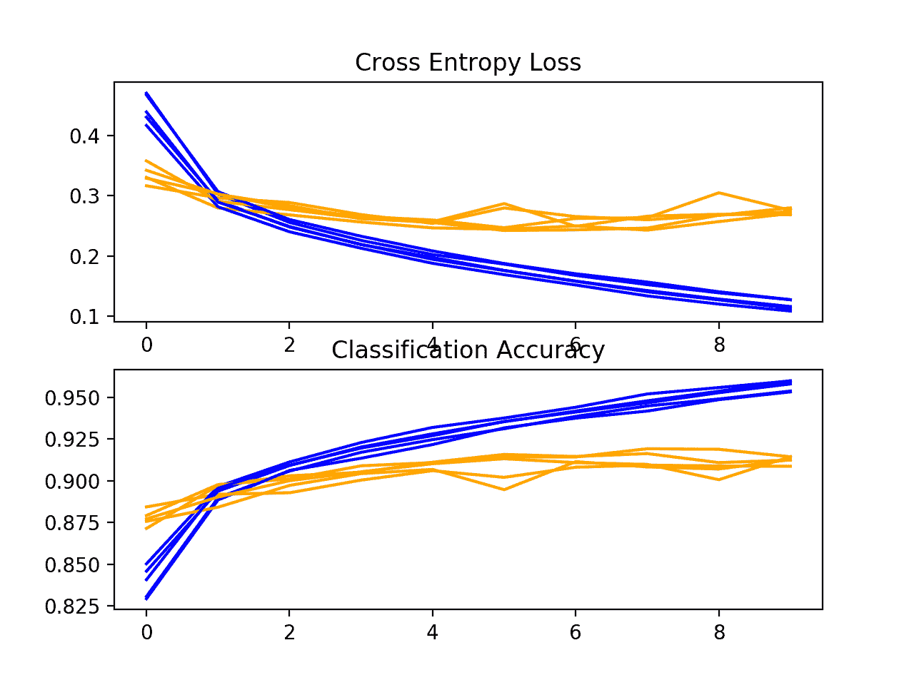
损失和准确性-学习曲线-相同填充-时尚-MNIST-数据集-在 k-折叠-交叉验证期间
接下来,给出了模型的估计表现,显示了模型的平均准确率非常轻微下降的表现,与基线模型的 91.187%相比,下降了 91.257%。
这可能是也可能不是真正的影响,因为它在标准偏差的范围内。也许更多的重复实验可以梳理出这个事实。
Accuracy: mean=91.257 std=0.209, n=5
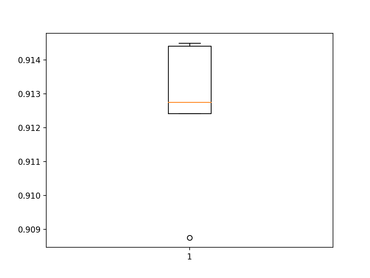
盒子和触须-准确度图-相同填充的分数-时尚-MNIST-数据集-评估-使用-k-折叠-交叉验证
增加过滤器
卷积层中使用的滤波器数量的增加通常可以提高表现,因为它可以为从输入图像中提取简单特征提供更多机会。
当使用非常小的滤波器时,例如 3×3 像素,这一点尤其重要。
在这个变化中,我们可以将卷积层的滤波器数量从 32 个增加到 64 个的两倍。我们还将通过使用“”相同的“”填充来建立可能的改进。
...
model.add(Conv2D(64, (3, 3), padding='same', activation='relu', kernel_initializer='he_uniform', input_shape=(28, 28, 1)))
为了完整起见,下面提供了完整的代码列表,包括对填充的更改。
# model with double the filters for the fashion mnist dataset
from numpy import mean
from numpy import std
from matplotlib import pyplot
from sklearn.model_selection import KFold
from keras.datasets import fashion_mnist
from keras.utils import to_categorical
from keras.models import Sequential
from keras.layers import Conv2D
from keras.layers import MaxPooling2D
from keras.layers import Dense
from keras.layers import Flatten
from keras.optimizers import SGD

# load train and test dataset
def load_dataset():
	# load dataset
	(trainX, trainY), (testX, testY) = fashion_mnist.load_data()
	# reshape dataset to have a single channel
	trainX = trainX.reshape((trainX.shape[0], 28, 28, 1))
	testX = testX.reshape((testX.shape[0], 28, 28, 1))
	# one hot encode target values
	trainY = to_categorical(trainY)
	testY = to_categorical(testY)
	return trainX, trainY, testX, testY

# scale pixels
def prep_pixels(train, test):
	# convert from integers to floats
	train_norm = train.astype('float32')
	test_norm = test.astype('float32')
	# normalize to range 0-1
	train_norm = train_norm / 255.0
	test_norm = test_norm / 255.0
	# return normalized images
	return train_norm, test_norm

# define cnn model
def define_model():
	model = Sequential()
	model.add(Conv2D(64, (3, 3), padding='same', activation='relu', kernel_initializer='he_uniform', input_shape=(28, 28, 1)))
	model.add(MaxPooling2D((2, 2)))
	model.add(Flatten())
	model.add(Dense(100, activation='relu', kernel_initializer='he_uniform'))
	model.add(Dense(10, activation='softmax'))
	# compile model
	opt = SGD(lr=0.01, momentum=0.9)
	model.compile(optimizer=opt, loss='categorical_crossentropy', metrics=['accuracy'])
	return model

# evaluate a model using k-fold cross-validation
def evaluate_model(dataX, dataY, n_folds=5):
	scores, histories = list(), list()
	# prepare cross validation
	kfold = KFold(n_folds, shuffle=True, random_state=1)
	# enumerate splits
	for train_ix, test_ix in kfold.split(dataX):
		# define model
		model = define_model()
		# select rows for train and test
		trainX, trainY, testX, testY = dataX[train_ix], dataY[train_ix], dataX[test_ix], dataY[test_ix]
		# fit model
		history = model.fit(trainX, trainY, epochs=10, batch_size=32, validation_data=(testX, testY), verbose=0)
		# evaluate model
		_, acc = model.evaluate(testX, testY, verbose=0)
		print('> %.3f' % (acc * 100.0))
		# append scores
		scores.append(acc)
		histories.append(history)
	return scores, histories

# plot diagnostic learning curves
def summarize_diagnostics(histories):
	for i in range(len(histories)):
		# plot loss
		pyplot.subplot(211)
		pyplot.title('Cross Entropy Loss')
		pyplot.plot(histories[i].history['loss'], color='blue', label='train')
		pyplot.plot(histories[i].history['val_loss'], color='orange', label='test')
		# plot accuracy
		pyplot.subplot(212)
		pyplot.title('Classification Accuracy')
		pyplot.plot(histories[i].history['accuracy'], color='blue', label='train')
		pyplot.plot(histories[i].history['val_accuracy'], color='orange', label='test')
	pyplot.show()

# summarize model performance
def summarize_performance(scores):
	# print summary
	print('Accuracy: mean=%.3f std=%.3f, n=%d' % (mean(scores)*100, std(scores)*100, len(scores)))
	# box and whisker plots of results
	pyplot.boxplot(scores)
	pyplot.show()

# run the test harness for evaluating a model
def run_test_harness():
	# load dataset
	trainX, trainY, testX, testY = load_dataset()
	# prepare pixel data
	trainX, testX = prep_pixels(trainX, testX)
	# evaluate model
	scores, histories = evaluate_model(trainX, trainY)
	# learning curves
	summarize_diagnostics(histories)
	# summarize estimated performance
	summarize_performance(scores)

# entry point, run the test harness
run_test_harness()
运行该示例会报告交叉验证过程中每个折叠的模型表现。
注:考虑到算法或评估程序的随机性,或数值准确率的差异,您的结果可能会有所不同。考虑运行该示例几次,并比较平均结果。
每倍分数可能表明比基线和单独使用相同的填充有一些进一步的改进。
> 90.917
> 90.908
> 90.175
> 91.158
> 91.408
创建了一个学习曲线的图,在这种情况下显示模型仍然对问题有合理的拟合,有一些运行过拟合的小迹象。
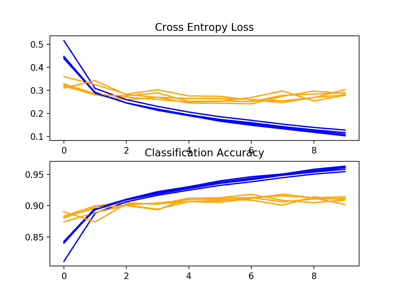
损失和准确性-学习曲线-更多-过滤器和填充-时尚-MNIST-数据集-k-折叠-交叉验证
接下来,给出了模型的估计表现,与基线相比,表现略有提高,从 90.913%提高到 91.257%。
同样,变化仍然在标准差的范围内,不清楚效果是否真实。
Accuracy: mean=90.913 std=0.412, n=5
如何最终确定模型并做出预测
只要我们有想法,有时间和资源来测试,模型改进的过程可能会持续很长时间。
在某些时候,必须选择并采用最终的模型配置。在这种情况下,我们将保持简单,并使用基线模型作为最终模型。
首先,我们将最终确定我们的模型,但是在整个训练数据集上拟合一个模型,并将该模型保存到文件中供以后使用。然后,我们将加载模型,并在等待测试数据集上评估其表现,以了解所选模型在实践中的实际表现。最后,我们将使用保存的模型对单个图像进行预测。
保存最终模型
最终模型通常适合所有可用数据,例如所有训练和测试数据集的组合。
在本教程中,我们有意保留一个测试数据集,以便我们可以估计最终模型的表现,这在实践中可能是一个好主意。因此,我们将只在训练数据集上拟合我们的模型。
# fit model
model.fit(trainX, trainY, epochs=10, batch_size=32, verbose=0)
一旦合适,我们可以通过调用模型上的 save() 函数将最终模型保存到一个 h5 文件中,并传入选择的文件名。
# save model
model.save('final_model.h5')
注意:保存和加载 Keras 模型需要在您的工作站上安装 h5py 库。
下面列出了在训练数据集上拟合最终模型并将其保存到文件中的完整示例。
# save the final model to file
from keras.datasets import fashion_mnist
from keras.utils import to_categorical
from keras.models import Sequential
from keras.layers import Conv2D
from keras.layers import MaxPooling2D
from keras.layers import Dense
from keras.layers import Flatten
from keras.optimizers import SGD

# load train and test dataset
def load_dataset():
	# load dataset
	(trainX, trainY), (testX, testY) = fashion_mnist.load_data()
	# reshape dataset to have a single channel
	trainX = trainX.reshape((trainX.shape[0], 28, 28, 1))
	testX = testX.reshape((testX.shape[0], 28, 28, 1))
	# one hot encode target values
	trainY = to_categorical(trainY)
	testY = to_categorical(testY)
	return trainX, trainY, testX, testY

# scale pixels
def prep_pixels(train, test):
	# convert from integers to floats
	train_norm = train.astype('float32')
	test_norm = test.astype('float32')
	# normalize to range 0-1
	train_norm = train_norm / 255.0
	test_norm = test_norm / 255.0
	# return normalized images
	return train_norm, test_norm

# define cnn model
def define_model():
	model = Sequential()
	model.add(Conv2D(32, (3, 3), activation='relu', kernel_initializer='he_uniform', input_shape=(28, 28, 1)))
	model.add(MaxPooling2D((2, 2)))
	model.add(Flatten())
	model.add(Dense(100, activation='relu', kernel_initializer='he_uniform'))
	model.add(Dense(10, activation='softmax'))
	# compile model
	opt = SGD(lr=0.01, momentum=0.9)
	model.compile(optimizer=opt, loss='categorical_crossentropy', metrics=['accuracy'])
	return model

# run the test harness for evaluating a model
def run_test_harness():
	# load dataset
	trainX, trainY, testX, testY = load_dataset()
	# prepare pixel data
	trainX, testX = prep_pixels(trainX, testX)
	# define model
	model = define_model()
	# fit model
	model.fit(trainX, trainY, epochs=10, batch_size=32, verbose=0)
	# save model
	model.save('final_model.h5')

# entry point, run the test harness
run_test_harness()
运行此示例后,您将在当前工作目录中拥有一个名为“ final_model.h5 ”的 1.2 兆字节文件。
评估最终模型
我们现在可以加载最终模型,并在等待测试数据集上对其进行评估。
如果我们有兴趣向项目涉众展示所选模型的表现,这是我们可以做的事情。
可通过 load_model() 功能加载模型。
下面列出了加载保存的模型并在测试数据集上对其进行评估的完整示例。
# evaluate the deep model on the test dataset
from keras.datasets import fashion_mnist
from keras.models import load_model
from keras.utils import to_categorical

# load train and test dataset
def load_dataset():
	# load dataset
	(trainX, trainY), (testX, testY) = fashion_mnist.load_data()
	# reshape dataset to have a single channel
	trainX = trainX.reshape((trainX.shape[0], 28, 28, 1))
	testX = testX.reshape((testX.shape[0], 28, 28, 1))
	# one hot encode target values
	trainY = to_categorical(trainY)
	testY = to_categorical(testY)
	return trainX, trainY, testX, testY

# scale pixels
def prep_pixels(train, test):
	# convert from integers to floats
	train_norm = train.astype('float32')
	test_norm = test.astype('float32')
	# normalize to range 0-1
	train_norm = train_norm / 255.0
	test_norm = test_norm / 255.0
	# return normalized images
	return train_norm, test_norm

# run the test harness for evaluating a model
def run_test_harness():
	# load dataset
	trainX, trainY, testX, testY = load_dataset()
	# prepare pixel data
	trainX, testX = prep_pixels(trainX, testX)
	# load model
	model = load_model('final_model.h5')
	# evaluate model on test dataset
	_, acc = model.evaluate(testX, testY, verbose=0)
	print('> %.3f' % (acc * 100.0))

# entry point, run the test harness
run_test_harness()
运行该示例将加载保存的模型,并在暂挂测试数据集上评估该模型。
计算并打印测试数据集中模型的分类准确率。
注:考虑到算法或评估程序的随机性,或数值准确率的差异,您的结果可能会有所不同。考虑运行该示例几次,并比较平均结果。
在这种情况下,我们可以看到模型达到了 90.990%的准确率,或者说仅仅是不到 10%的分类误差,这还不错。
> 90.990
作出预测
我们可以使用保存的模型对新图像进行预测。
该模型假设新图像是灰度的,它们已经被分割,使得一幅图像包含黑色背景上的一件居中的衣服,并且图像的大小是 28×28 像素的正方形。
下面是从 MNIST 测试数据集中提取的图像。您可以将其保存在当前工作目录中,文件名为“ sample_image.png ”。
样品服装(套头衫)
我们将假装这是一个全新的、看不见的图像,按照要求的方式准备,看看我们如何使用保存的模型来预测图像所代表的整数。对于这个例子,我们期望类“ 2 ”用于“套头衫”(也称为套头衫)。
首先,我们可以加载图像,强制为灰度格式,并强制大小为 28×28 像素。然后,可以调整加载图像的大小,使其具有单个通道,并表示数据集中的单个样本。 load_image() 函数实现了这一点,并将返回已加载的准备分类的图像。
重要的是,像素值的准备方式与在拟合最终模型时为训练数据集准备像素值的方式相同,在这种情况下,最终模型是归一化的。
# load and prepare the image
def load_image(filename):
	# load the image
	img = load_img(filename, grayscale=True, target_size=(28, 28))
	# convert to array
	img = img_to_array(img)
	# reshape into a single sample with 1 channel
	img = img.reshape(1, 28, 28, 1)
	# prepare pixel data
	img = img.astype('float32')
	img = img / 255.0
	return img
接下来,我们可以像上一节一样加载模型,并调用*predict _ class()*函数来预测图像中的服装。
# predict the class
result = model.predict_classes(img)
下面列出了完整的示例。
# make a prediction for a new image.
from keras.preprocessing.image import load_img
from keras.preprocessing.image import img_to_array
from keras.models import load_model

# load and prepare the image
def load_image(filename):
	# load the image
	img = load_img(filename, grayscale=True, target_size=(28, 28))
	# convert to array
	img = img_to_array(img)
	# reshape into a single sample with 1 channel
	img = img.reshape(1, 28, 28, 1)
	# prepare pixel data
	img = img.astype('float32')
	img = img / 255.0
	return img

# load an image and predict the class
def run_example():
	# load the image
	img = load_image('sample_image.png')
	# load model
	model = load_model('final_model.h5')
	# predict the class
	result = model.predict_classes(img)
	print(result[0])

# entry point, run the example
run_example()
运行该示例首先加载和准备图像,加载模型,然后正确预测加载的图像代表套头衫或“2”类。
2
扩展ˌ扩张
本节列出了一些您可能希望探索的扩展教程的想法。
- 正规化。探索与基线模型相比,添加正则化如何影响模型表现,例如权重衰减、提前停止和退出。
- 调整学习率。探究与基线模型相比,不同的学习率如何影响模型表现,例如 0.001 和 0.0001。
- 调整模型深度。探索与基线模型相比,向模型中添加更多层如何影响模型表现,例如模型的分类器部分中的另一个卷积和池层块或另一个密集层。
如果你探索这些扩展,我很想知道。
在下面的评论中发表你的发现。
进一步阅读
如果您想更深入地了解这个主题,本节将提供更多资源。
蜜蜂
文章
摘要
在本教程中,您发现了如何从零开始开发用于服装分类的卷积神经网络。
具体来说,您了解到:
- 如何开发一个测试工具来开发一个健壮的模型评估,并为分类任务建立一个表现基线。
- 如何探索基线模型的扩展,以提高学习和模型能力。
- 如何开发最终模型,评估最终模型的表现,并使用它对新图像进行预测。
你有什么问题吗?
在下面的评论中提问,我会尽力回答。


 1433
1433

 被折叠的 条评论
为什么被折叠?
被折叠的 条评论
为什么被折叠?
 到【灌水乐园】发言


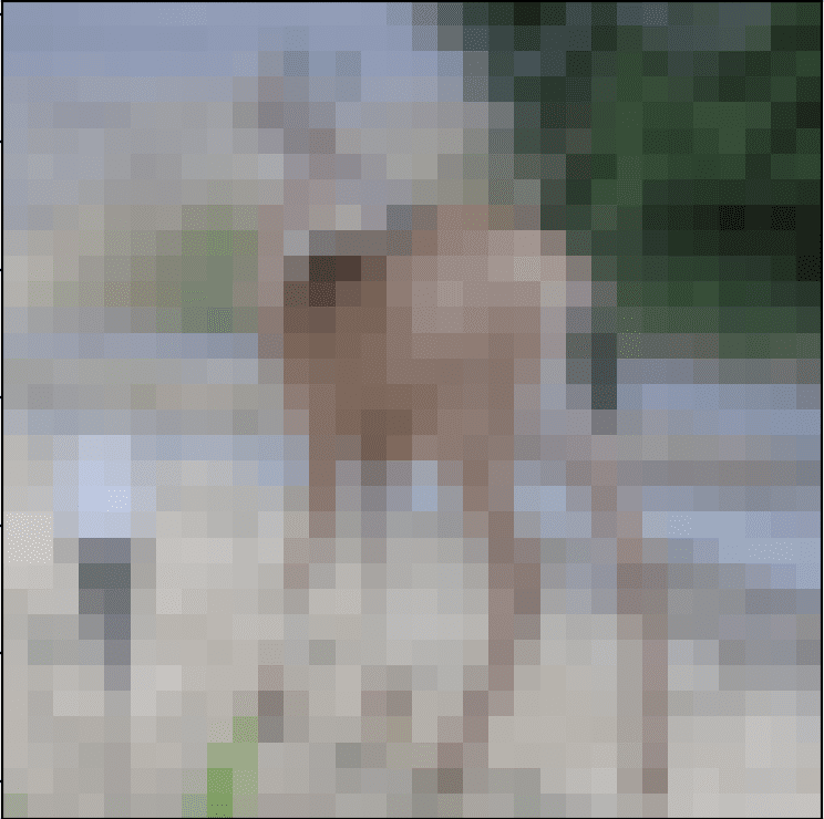