终于来了！智能优化算法之收敛过程动态图

声明：对于作者的原创代码，禁止转售倒卖，违者必究！

智能优化算法的文章中，为了对比算法的收敛速度，经常会在论文中放置关于粒子迭代过程的位置分布图，形如这样：

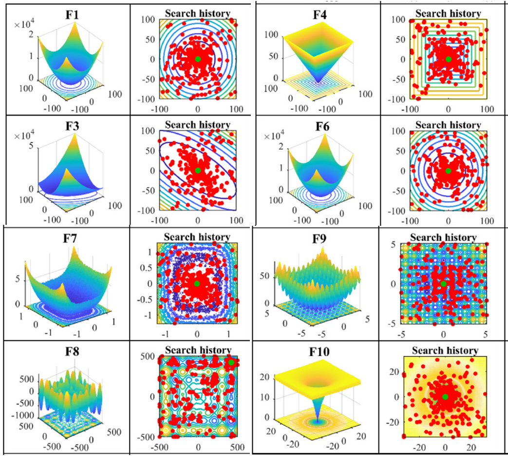
今天咱们就复现一下这种位置动态分布图！以粒子群算法为例(其他算法都非常好替换哦！直接对照粒子群的案例即可简单替换！)，在CEC2005函数集中进行展示：

F1：

F2:

F3:

F4:

F7:

F8:

F9:

F10:

F12:

部分代码展示：

%%
clear
clc
close all
addpath(genpath(pwd));
number='F1'; %选定优化函数，自行替换:F1~F23
[lower_bound,upper_bound,variables_no,fobj]=Get_Functions_details(number);  % [lb,ub,D,y]：下界、上界、维度、目标函数表达式
pop_size=100;                      % population members
max_iter=50;                  % maximum number of iteration
%% PSO
[PSO_Best_score,Best_pos,PSO_curve,HistoryPosition,HistoryBest]=PSO(pop_size,max_iter,lower_bound,upper_bound,variables_no,fobj);  % Calculating the solution of the given problem using PSO
display(['The best optimal value of the objective funciton found by PSO  for ' [num2str(number)],'  is : ', num2str(PSO_Best_score)]);


%% Figure
figure1 = figure('Color',[1 1 1]);
G1=subplot(1,2,1,'Parent',figure1);
func_plot(number)
title(number)
xlabel('x')
ylabel('y')
zlabel('z')
subplot(1,2,2)
CNT=20;
k=round(linspace(1,max_iter,CNT)); %随机选CNT个点
% 注意：如果收敛曲线画出来的点很少，随机点很稀疏，说明点取少了，这时应增加取点的数量，100、200、300等，逐渐增加
% 相反，如果收敛曲线上的随机点非常密集，说明点取多了，此时要减少取点数量
iter=1:1:max_iter;
if ~strcmp(number,'F16')&&~strcmp(number,'F9')&&~strcmp(number,'F11')  %这里是因为这几个函数收敛太快，不适用于semilogy，直接plot
    semilogy(iter(k),PSO_curve(k),'g-x','linewidth',1);
else
    plot(iter(k),PSO_curve(k),'g-x','linewidth',1);
end
grid on;
title('收敛曲线')
xlabel('迭代次数');
ylabel('适应度值');
box on
legend('PSO')
set (gcf,'position', [300,300,800,330])


%% 绘制每一代粒子群距离的分布
for i = 1:max_iter
    Position = HistoryPosition{i};%获取当前代位置
    BestPosition = HistoryBest{i};%获取当前代最佳位置
    figure(3)
    funcplot(number)
    hold on
    plot(Position(:,1),Position(:,2),'b*','linewidth',3);
    hold on;
    plot(BestPosition(1),BestPosition(2),'rp','linewidth',3);
    grid on;
    if length(lower_bound)==1 
        axis ([lower_bound upper_bound lower_bound upper_bound])
    else
        axis ([lower_bound(1) upper_bound(1) lower_bound(2) upper_bound(2)])
    end
    legend('投影图','粒子群位置','最佳粒子群距离值');
    title(['第',num2str(i),'次迭代']);
    hold off
end

代码目录

运行Main.m即可。

代码获取方式：下方支付后会显示网盘链接！