机器学习之信用卡欺诈案例(混淆矩阵、数据预处理、模型评估）

1.案例背景

1. 数据说明：这一份数据是信用卡的消费使用数据，其中数据涉及到一些隐私的内容，里面的相关数据特征已经经过了处理，我们拿到的数据并不是最原始的数据。我们通过逻辑回归来预测信用卡异常的数据。

2. 观察数据

   代码：

   import pandas as pd
   import numpy as np
   import matplotlib.pyplot as plt
   
   data = pd.read_csv('data/creditcard.csv')
   data.head()
   print(data)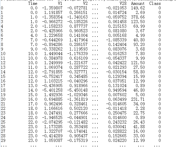
   

   

   ​ time 对我们来说是没有用的，我们待会会将这一部分去掉。amount代表着交易的金额。在V1~V28 的数据比较小，而amount数据都比较大，所以要对数据进行预处理操作。

   ​ 属于0 这个类是正常的，属于1 这个类是异常的。我们的目的是进行分类任务。绝大多数样本是正样本，少数样本是负样本。

   2.样本不平衡的解决方案

   #  观察样本的分布规则
   count_classes = pd.value_counts(data['Class'],sort=True)
   count_classes.plot(kind='bar')
   plt.title("Fraud class histogram")
   plt.xlabel("Class")
   plt.ylabel("Frequency")
   plt.show()
   

   ​

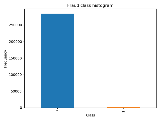
   ​ 从中可以观察到，正负样本不均衡。

   ​ 这里有两种解决方案：1.下采样 ：让0和1 两个样本一样小 2. 过采样： 对1号 样本进行生成，让 0 和 1 这两个样本一样多。

   ​ 我们在这里并没有说amount特征比较重要，所以这里先进行归一化操作！

   from sklearn.preprocessing import StandardScaler
   data['normAmount'] = StandardScaler().fit_transform(data['Amount'].values.reshape(-1, 1))
   data = data.drop(['Time','Amount'],axis=1)
   print(data.head())
   

   ​

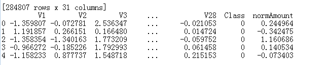
   ​ 这里得到了我们可以直接使用的特征数据。

   • 下采样策略

     # 下采样，使得两个样本同样少
     X = data.ix[:, data.columns != 'Class']
     y = data.ix[:, data.columns == 'Class']
     
     # Number of data points in the minority class
     number_records_fraud = len(data[data.Class == 1])# 计算异常样本的个数
     fraud_indices = np.array(data[data.Class == 1].index) # 异常样本在原数据的索引值
     
     # Picking the indices of the normal classes
     normal_indices = data[data.Class == 0].index # 获得原数据正常样本的索引值
     
     # Out of the indices we picked, randomly select "x" number (number_records_fraud)
     random_normal_indices = np.random.choice(normal_indices, number_records_fraud, replace = False) # 通过索引进行随机的选择
     random_normal_indices = np.array(random_normal_indices)
     
     # Appending the 2 indices
     under_sample_indices = np.concatenate([fraud_indices,random_normal_indices]) # 将class=1和class=0 的选出来的索引值进行合并
     
     # Under sample dataset
     under_sample_data = data.iloc[under_sample_indices,:]
     
     X_undersample = under_sample_data.ix[:, under_sample_data.columns != 'Class']
     y_undersample = under_sample_data.ix[:, under_sample_data.columns == 'Class']
     
     # Showing ratio
     print("Percentage of normal transactions: ", len(under_sample_data[under_sample_data.Class == 0])/len(under_sample_data))
     print("Percentage of fraud transactions: ", len(under_sample_data[under_sample_data.Class == 1])/len(under_sample_data))
     print("Total number of transactions in resampled data: ", len(under_sample_data))
     

     Percentage of normal transactions: 0.5
     Percentage of fraud transactions: 0.5
     Total number of transactions in resampled data: 984

3.交叉验证

• 目的

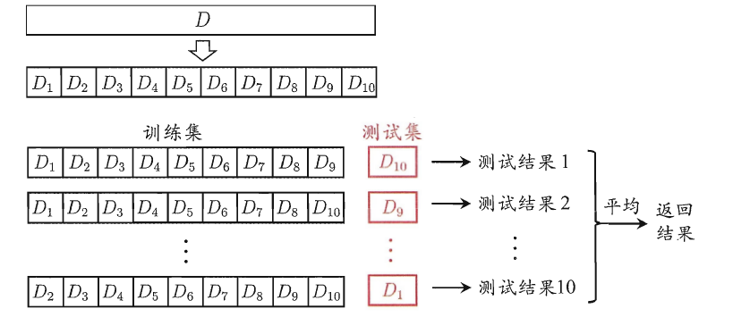
  交叉验证法的作用就是尝试利用不同的训练集/验证集划分来对模型做多组不同的训练/验证，来应对单独测试结果过于片面以及训练数据不足的问题。（就像通过多次考试，才通知哪些学生是比较比较牛B的）

  交叉验证的做法就是将数据集粗略地分为比较均等不相交的k份，然后取其中的一份进行测试，另外的k-1份进行训练，然后求得error的平均值作为最终的评价，具体算法流程如下：

  

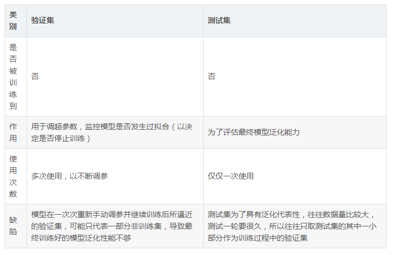
• 在有监督(supervise)的机器学习中，数据集常被分成2~3个，即：训练集(train set)，验证集(validation set)，测试集(test set)

  

  一个形象的比喻：

  **训练集-----------**学生的课本；学生 根据课本里的内容来掌握知识。

  验证集------------作业，通过作业可以知道 不同学生学习情况、进步的速度快慢。

  测试集-----------考试，考的题是平常都没有见过，考察学生举一反三的能力。

  传统上，一般三者切分的比例是：6：2：2，验证集并不是必须的。

  为什么要测试集

  a)训练集直接参与了模型调参的过程，显然不能用来反映模型真实的能力（防止课本死记硬背的学生拥有最好的成绩，即防止过拟合)

  b)验证集参与了人工调参(超参数)的过程，也不能用来最终评判一个模型（刷题库的学生不能算是学习好的学生）。

  c) 所以要通过最终的考试(测试集)来考察一个学(模)生(型)真正的能力**（期末考试）**

  但是仅凭一次考试就对模型的好坏进行评判显然是不合理的，所以接下来就要介绍交叉验证法

  from sklearn.model_selection import train_test_split
  
  # Whole dataset
  X_train, X_test, y_train, y_test = train_test_split(X,y,test_size = 0.3, random_state = 0)
  
  print("Number transactions train dataset: ", len(X_train))
  print("Number transactions test dataset: ", len(X_test))
  print("Total number of transactions: ", len(X_train)+len(X_test))
  
  # Undersampled dataset
  X_train_undersample, X_test_undersample, y_train_undersample, y_test_undersample = train_test_split(X_u