信用卡欺诈检测案例 -- 机器学习项目基础篇（2）

这个案例面临的挑战是识别欺诈性信用卡交易，以便信用卡公司的客户不会因为他们没有购买的物品而被收取费用。

信用卡欺诈检测中涉及的主要挑战是：

1. 每天都要处理大量数据，模型构建必须足够快，以便及时响应骗局。
2. 不平衡的数据，即大多数交易（99.8%）不是欺诈性的，这使得检测欺诈性交易变得非常困难。
3. 数据可用性，因为数据大部分是私有的。
4. 错误分类的数据可能是另一个主要问题，因为并非每一笔欺诈性交易都被捕获和报告。
5. 骗子对模型使用的自适应技术。

如何应对这些挑战？

1. 使用的模型必须足够简单和快速，以检测异常并尽快将其分类为欺诈交易。
2. 不平衡可以通过适当地使用一些方法来处理，我们将在下一段中讨论这些方法。
3. 为了保护用户的隐私，可以减少数据的维度。
4. 必须采用更可靠的来源，对数据进行双重检查，至少用于训练模型。
5. 我们可以让模型变得简单和可解释，这样当骗子通过一些调整来适应它时，我们就可以有一个新的模型来部署。

以下代码均在jupyter notebook中工作。
您可以从此链接下载数据集 https://www.kaggle.com/datasets/mlg-ulb/creditcardfraud

导入所有必要的库

# import the necessary packages
import numpy as np
import pandas as pd
import matplotlib.pyplot as plt
import seaborn as sns
from matplotlib import gridspec

加载数据

data = pd.read_csv("credit.csv")

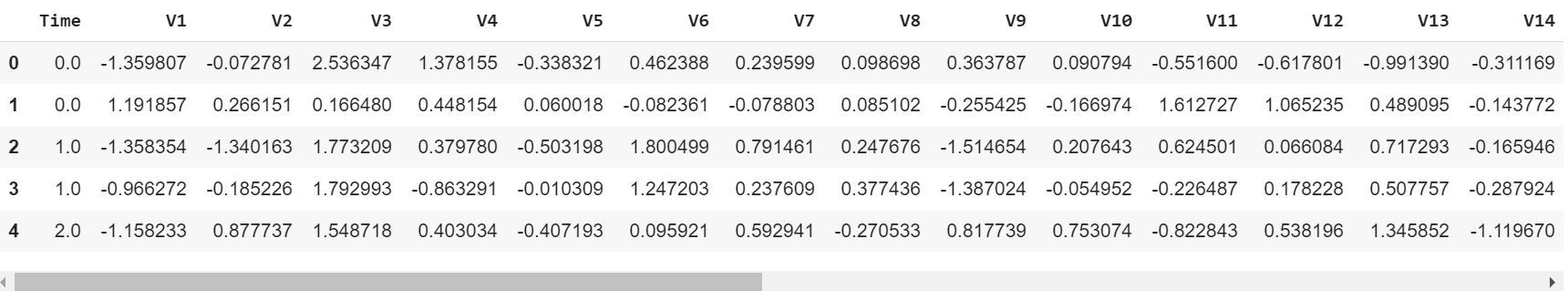
展示数据

data.head()

描述数据

print(data.shape)
print(data.describe())

是时候解释我们正在处理的数据了。

fraud = data[data['Class'] == 1]
valid = data[data['Class'] == 0]
outlierFraction = len(fraud)/float(len(valid))
print(outlierFraction)
print('Fraud Cases: {}'.format(len(data[data['Class'] == 1])))
print('Valid Transactions: {}'.format(len(data[data['Class'] == 0])))

只有0.17%的欺诈交易。数据非常不平衡。让我们首先应用我们的模型，而不平衡它，如果我们没有得到一个很好的准确性，那么我们可以找到一种方法来平衡这个数据集。但首先，让我们在没有它的情况下实现模型，并仅在需要时平衡数据。

打印欺诈交易的金额详情

print(“Amount details of the fraudulent transaction”)
fraud.Amount.describe()

输出：

Amount details of the fraudulent transaction
count     492.000000
mean      122.211321
std       256.683288
min         0.000000
25%         1.000000
50%         9.250000
75%       105.890000
max      2125.870000
Name: Amount, dtype: float64

打印正常交易的金额明细

print(“details of valid transaction”)
valid.Amount.describe()

Amount details of valid transaction
count    284315.000000
mean         88.291022
std         250.105092
min           0.000000
25%           5.650000
50%          22.000000
75%          77.050000
max       25691.160000
Name: Amount, dtype: float64

正如我们可以清楚地注意到，欺诈者的平均货币交易更多。这使得这个问题至关重要的处理。

绘制相关矩阵

相关性矩阵以图形方式为我们提供了特征如何相互关联的概念，并可以帮助我们预测哪些特征与预测最相关。

# Correlation matrix
corrmat = data.corr()
fig = plt.figure(figsize = (12, 9))
sns.heatmap(corrmat, vmax = .8, square = True)
plt.show()

在HeatMap中，我们可以清楚地看到，大多数特征与其他特征不相关，但有一些特征彼此之间具有正相关性或负相关性。例如，V2和V5与称为Amount的特征高度负相关。我们还看到与V20和Amount的一些相关性。这使我们对我们可用的数据有了更深入的了解。

分隔X和Y值

将数据划分为输入参数和输出值格式

# dividing the X and the Y from the dataset
X = data.drop(['Class'], axis = 1)
Y = data["Class"]
print(X.shape)
print(Y.shape)
# getting just the values for the sake of processing 
# (its a numpy array with no columns)
xData = X.values
yData = Y.values

输出：

(284807, 30)
(284807, )

训练和测试数据划分

我们将把数据集分成两个主要组。一个用于训练模型，另一个用于测试训练模型的性能。

# Using Scikit-learn to split data into training and testing sets
from sklearn.model_selection import train_test_split
# Split the data into training and testing sets
xTrain, xTest, yTrain, yTest = train_test_split(
        xData, yData, test_size = 0.2, random_state = 42)

使用scikit learn构建随机森林模型

from sklearn.ensemble import RandomForestClassifier
# random forest model creation
rfc = RandomForestClassifier()
rfc.fit(xTrain, yTrain)
# predictions
yPred = rfc.predict(xTest)

建立各种评价参数

# Evaluating the classifier
# printing every score of the classifier
# scoring in anything
from sklearn.metrics import classification_report, accuracy_score 
from sklearn.metrics import precision_score, recall_score
from sklearn.metrics import f1_score, matthews_corrcoef
from sklearn.metrics import confusion_matrix
  
n_outliers = len(fraud)
n_errors = (yPred != yTest).sum()
print("The model used is Random Forest classifier")
  
acc = accuracy_score(yTest, yPred)
print("The accuracy is {}".format(acc))
  
prec = precision_score(yTest, yPred)
print("The precision is {}".format(prec))
  
rec = recall_score(yTest, yPred)
print("The recall is {}".format(rec))
  
f1 = f1_score(yTest, yPred)
print("The F1-Score is {}".format(f1))
  
MCC = matthews_corrcoef(yTest, yPred)
print("The Matthews correlation coefficient is{}".format(MCC))

输出：

The model used is Random Forest classifier
The accuracy is  0.9995611109160493
The precision is 0.9866666666666667
The recall is 0.7551020408163265
The F1-Score is 0.8554913294797689
The Matthews correlation coefficient is0.8629589216367891

可视化混淆矩阵

# printing the confusion matrix
LABELS = ['Normal', 'Fraud']
conf_matrix = confusion_matrix(yTest, yPred)
plt.figure(figsize =(12, 12))
sns.heatmap(conf_matrix, xticklabels = LABELS, 
            yticklabels = LABELS, annot = True, fmt ="d");
plt.title("Confusion matrix")
plt.ylabel('True class')
plt.xlabel('Predicted class')
plt.show()

与其他算法进行比较，不处理数据的不平衡性。

正如你可以看到我们的随机森林模型，我们得到了一个更好的结果，即使是最棘手的召回部分。