


 文章详细介绍了StableDiffusionPipeline中的各个组件,如VAE、UNet、调度器等,并展示了如何在生成图像时运用这些组件。内容涵盖了模型结构、编码解码、文本控制和不同Pipeline的应用实例。
推荐阅读列表:
扩散模型实战(十):Stable Diffusion文本条件生成图像大模型
在扩散模型实战(十):Stable Diffusion文本条件生成图像大模型中介绍了如何使用Stable Diffusion Pipeline控制图片生成效果以及大小,本文让我们剖析一下Stable Diffusion Pipeline内容细节。
Stable Diffusion Pipeline要比之前介绍的DDPMPipeline复杂一些,除了UNet和调度器还有其他组件,让我们来看一下具体包括的组件:
from diffusers import (StableDiffusionPipeline,StableDiffusionImg2ImgPipeline,StableDiffusionInpaintPipeline,StableDiffusionDepth2ImgPipeline)
# 载入管线model_id = "stabilityai/stable-diffusion-2-1-base"pipe = StableDiffusionPipeline.from_pretrained(model_id).to(device)pipe = StableDiffusionPipeline.from_pretrained(model_id,revision="fp16",torch_dtype=torch.float16).to(device)
# 查看pipe的组件print(list(pipe.components.keys()))
# 输出组件['vae','text_encoder','tokenizer','unet','scheduler','safety_checker','feature_extractor']
这些组件的概念之前都介绍过了,下面通过代码分析一下这些组件的细节:
一、可变分自编码器(VAE)
可变分自编码器(VAE)是一种模型,模型结构如图所示:
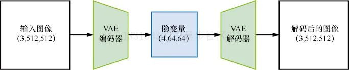
在使用Stable Diffusion生成图片时,首先需要在VAE的“隐空间”中应用扩散过程以生成隐编码,然后在扩散之后对他们解码,得到最终的输出图片,实际上,UNet的输入不是完整的图片,而是经过VAE压缩后的特征,这样可以极大地减少计算资源,代码如下:
# 创建取值区间为(-1, 1)的伪数据images = torch.rand(1, 3, 512, 512).to(device) * 2 - 1print("Input images shape:", images.shape)# 编码到隐空间with torch.no_grad():latents = 0.18215 * pipe.vae.encode(images).latent_dist.meanprint("Encoded latents shape:", latents.shape)# 再解码回来with torch.no_grad():decoded_images = pipe.vae.decode(latents / 0.18215).sampleprint("Decoded images shape:", decoded_images.shape)
# 输出Input images shape: torch.Size([1, 3, 512, 512])Encoded latents shape: torch.Size([1, 4, 64, 64])Decoded images shape: torch.Size([1, 3, 512, 512])
在这个示例中,原本512X512像素的图片被压缩成64X64的隐式表示,图片的每个空间维度都被压缩至原来的八分之一,因此设定参数width和height时,需要将它们设置成8的倍数。
PS:VAE解码过程并不完美,图像质量有所损失,但在实际使用中已经足够好了。
二、分词器tokenizer和文本编码器text_encoder
Prompt文本描述如何控制Stable Diffusion呢?首先需要对Prompt文本描述使用tokenizer进行分词转换为数值表示的ID,然后将这些分词后的ID输入给文本编码器。实际使用户中,可以直接调用_encode_prompt方法来补全或者截断分词后的长度为77获得最终的Prompt文本表示,代码如下:
# 手动对提示文字进行分词和编码# 分词input_ids = pipe.tokenizer(["A painting of a flooble"])['input_ids']print("Input ID -> decoded token")for input_id in input_ids[0]:print(f"{input_id} -> {pipe.tokenizer.decode(input_id)}")# 将分词结果输入CLIPinput_ids = torch.tensor(input_ids).to(device)with torch.no_grad():text_embeddings = pipe.text_encoder(input_ids)['last_hidden_state']print("Text embeddings shape:", text_embeddings.shape)
# 输出Input ID -> decoded token49406 -> <|startoftext|>320 -> a3086 -> painting539 -> of320 -> a4062 -> floo1059 -> ble49407 -> <|endoftext|>Text embeddings shape: torch.Size([1, 8, 1024])
获取最终的文本特征
text_embeddings = pipe._encode_prompt("A painting of a flooble",device, 1, False, '')print(text_embeddings.shape)
# 输出torch.Size([1, 77, 1024])
可以看到最终的文本从长度8补全到了77。
三、UNet网络
在扩散模型中,UNet的作用是接收“带噪”的输入并预测噪声,以实现“去噪”,网络结构如下图所示,与前面的示例不同,此次输入的并非是原始图片,而是图片的隐式表示,另外还有文本Prompt描述也作为UNet的输入。
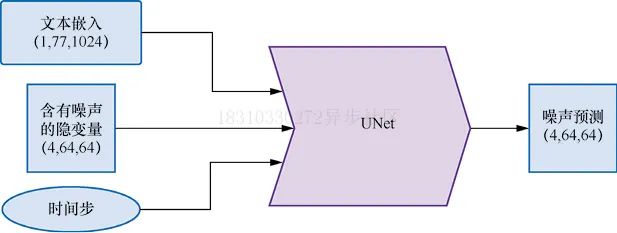
下面让我们对上述三种输入使用伪输入让模型来了解一下UNet在预测过程中,输入输出形状和大小,代码如下:
# 创建伪输入timestep = pipe.scheduler.timesteps[0]latents = torch.randn(1, 4, 64, 64).to(device)text_embeddings = torch.randn(1, 77, 1024).to(device)# 让模型进行预测with torch.no_grad():unet_output = pipe.unet(latents, timestep, text_embeddings).sampleprint('UNet output shape:', unet_output.shape)
# 输出UNet output shape: torch.Size([1, 4, 64, 64])
四、调度器Scheduler
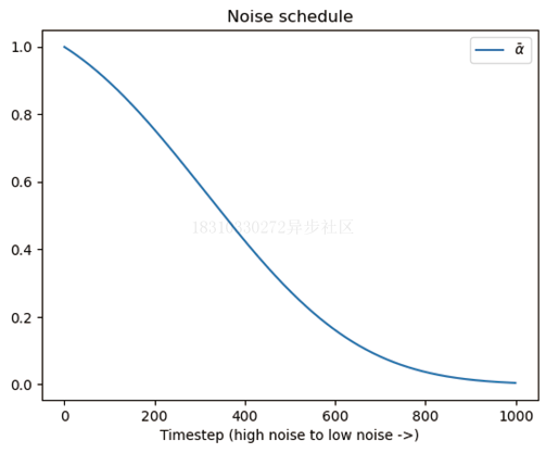
调度器保持了如何添加噪声的信息,并管理如何基于模型的预测更新“带噪”样本,默认的调度器是PNDMScheduler。
我们可以观察一下在添加噪声过程中,噪声水平随时间步增加的变化
plt.plot(pipe.scheduler.alphas_cumprod, label=r'$\bar{\alpha}$')plt.xlabel('Timestep (high noise to low noise ->)')plt.title('Noise schedule')plt.legend()
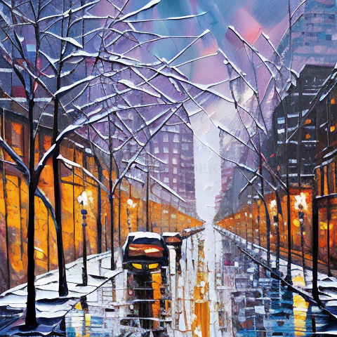
下面看一下使用不同的调度器生成的效果对比,比如使用LMSDiscreteScheduler,代码如下:
from diffusers import LMSDiscreteScheduler# 替换原来的调度器pipe.scheduler = LMSDiscreteScheduler.from_config(pipe.scheduler.config)# 输出配置参数print('Scheduler config:', pipe.scheduler)# 使用新的调度器生成图片pipe(prompt="Palette knife painting of an winter cityscape",height=480, width=480, generator=torch.Generator(device=device).manual_seed(42)).images[0]
# 输出Scheduler config: LMSDiscreteScheduler {"_class_name": "LMSDiscreteScheduler","_diffusers_version": "0.11.1","beta_end": 0.012,"beta_schedule": "scaled_linear","beta_start": 0.00085,"clip_sample": false,"num_train_timesteps": 1000,"prediction_type": "epsilon","set_alpha_to_one": false,"skip_prk_steps": true,"steps_offset": 1,"trained_betas": null}
生成的图片如下图所示:
五、复现完整Pipeline
到目前为止,我们已经分步骤剖析了Pipeline的每个组件,现在我们将组合起来手动实现一个完整的Pipeline,代码如下:
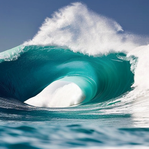
guidance_scale = 8num_inference_steps=30prompt = "Beautiful picture of a wave breaking"negative_prompt = "zoomed in, blurry, oversaturated, warped"# 对提示文字进行编码text_embeddings = pipe._encode_prompt(prompt, device, 1, True,negative_prompt)# 创建随机噪声作为起点latents = torch.randn((1, 4, 64, 64), device=device, generator=generator)latents *= pipe.scheduler.init_noise_sigma# 准备调度器pipe.scheduler.set_timesteps(num_inference_steps, device=device)# 生成过程开始for i, t in enumerate(pipe.scheduler.timesteps):latent_model_input = torch.cat([latents] * 2)latent_model_input = pipe.scheduler.scale_model_input(latent_model_input, t)with torch.no_grad():noise_pred = pipe.unet(latent_model_input, t,encoder_hidden_states=text_embeddings).samplenoise_pred_uncond, noise_pred_text = noise_pred.chunk(2)noise_pred = noise_pred_uncond + guidance_scale *(noise_pred_text - noise_pred_uncond)latents = pipe.scheduler.step(noise_pred, t, latents).prev_sample# 将隐变量映射到图片,效果如图6-14所示with torch.no_grad():image = pipe.decode_latents(latents.detach())pipe.numpy_to_pil(image)[0]
生成的效果,如下图所示:
六、其他Pipeline介绍
在也提到一些其他Pipeline模型,比如图片到图片风格迁移Img2Img,图片修复Inpainting以及图片深度Depth2Image模型,本小节我们就来探索一下这些模型的具体使用效果。
6.1 Img2Img
到目前为止,我们的图片仍然是从完全随机的隐变量开始生成的,并且都使用了完整的扩展模型采样循环。Img2Img Pipeline不必从头开始,它首先会对一张已有的图片进行编码,在得到一系列的隐变量后,就在这些隐变量上随机添加噪声,并以此作为起点。
噪声的数量和“去噪”的步数决定了Img2Img生成的效果,添加少量噪声只会带来微小的变化,添加大量噪声并执行完整的“去噪”过程,可能得到与原始图片完全不同,近在整体结构上相似的图片。
# 载入Img2Img管线model_id = "stabilityai/stable-diffusion-2-1-base"img2img_pipe = StableDiffusionImg2ImgPipeline.from_pretrained(model_id).to(device)
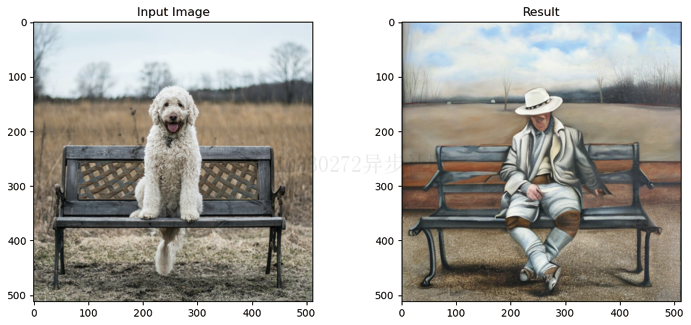
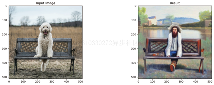
result_image = img2img_pipe(prompt="An oil painting of a man on a bench",image = init_image, # 输入待编辑图片strength = 0.6, # 文本提示在设为0时完全不起作用,设为1时作用强度最大).images[0]# 显示结果,如图6-15所示fig, axs = plt.subplots(1, 2, figsize=(12, 5))axs[0].imshow(init_image);axs[0].set_title('Input Image')axs[1].imshow(result_image);axs[1].set_title('Result')
生成的效果,如下图所示:
6.2 Inpainting
Inpainting是一个图片修复技术,它可以保留图片一部分内容不变,其他部分生成新的内容,Inpainting UNet网络结构如下图所示:
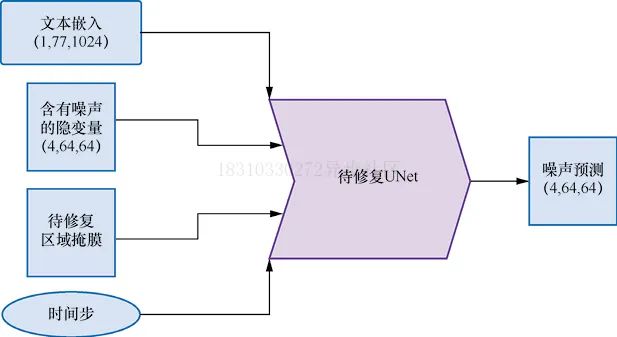
下面我们使用一个示例来展示一下效果:
pipe = StableDiffusionInpaintPipeline.from_pretrained("runwayml/stable-diffusion-inpainting")pipe = pipe.to(device)# 添加提示文字,用于让模型知道补全图像时使用什么内容prompt = "A small robot, high resolution, sitting on a park bench"image = pipe(prompt=prompt, image=init_image,mask_image=mask_image).images[0]# 查看结果,如图6-17所示fig, axs = plt.subplots(1, 3, figsize=(16, 5))axs[0].imshow(init_image);axs[0].set_title('Input Image')axs[1].imshow(mask_image);axs[1].set_title('Mask')axs[2].imshow(image);axs[2].set_title('Result')
生成的效果,如下图所示:
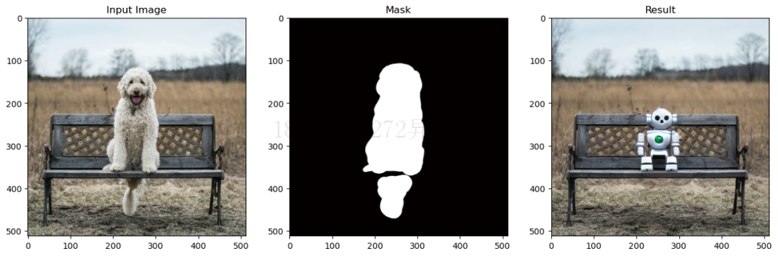
这是个有潜力的模型,如果可以和自动生成掩码的模型结合就会非常强大,比如Huggingface Space上的一个名为CLIPSeg的模型就可以自动生成掩码。
6.3 Depth2Image
如果想保留图片的整体结构而不保留原有的颜色,比如使用不同的颜色或纹理生成新图片,Img2Img是很难通过“强度”来控制的。而Depth2Img采用深度预测模型来预测一个深度图,这个深度图被输入微调过的UNet以生成图片,我们希望生成的图片既能保留原始图片的深度信息和总体结构,同时又能在相关部分填入全新的内容,代码如下:
# 载入Depth2Img管线pipe = StableDiffusionDepth2ImgPipeline.from_pretrained("stabilityai/stable-diffusion-2-depth")pipe = pipe.to(device)# 使用提示文字进行图像补全prompt = "An oil painting of a man on a bench"image = pipe(prompt=prompt, image=init_image).images[0]# 查看结果,如图6-18所示fig, axs = plt.subplots(1, 2, figsize=(16, 5))axs[0].imshow(init_image);axs[0].set_title('Input Image')axs[1].imshow(image);axs[1].set_title('Result')
PS:该模型在3D场景下加入纹理非常有用。


 782
782

 被折叠的 条评论
为什么被折叠?
被折叠的 条评论
为什么被折叠?
 到【灌水乐园】发言


