扩散模型实战（十二）：使用调度器DDIM反转来优化图像编辑

 推荐阅读列表：

 扩散模型实战（一）：基本原理介绍

扩散模型实战（二）：扩散模型的发展

扩散模型实战（三）：扩散模型的应用

扩散模型实战（四）：从零构建扩散模型

扩散模型实战（五）：采样过程

扩散模型实战（六）：Diffusers DDPM初探

扩散模型实战（七）：Diffusers蝴蝶图像生成实战

扩散模型实战（八）：微调扩散模型

扩散模型实战（九）：使用CLIP模型引导和控制扩散模型

扩散模型实战（十）：Stable Diffusion文本条件生成图像大模型

扩散模型实战（十一）：剖析Stable Diffusion Pipeline各个组件

一、配置环境

# !pip install -q transformers diffusers accelerateimport torchimport requestsimport torch.nn as nnimport torch.nn.functional as Ffrom PIL import Imagefrom io import BytesIOfrom tqdm.auto import tqdmfrom matplotlib import pyplot as pltfrom torchvision import transforms as tfmsfrom diffusers import StableDiffusionPipeline, DDIMScheduler# 定义接下来将要用到的函数def load_image(url, size=None):    response = requests.get(url,timeout=0.2)    img = Image.open(BytesIO(response.content)).convert('RGB')    if size is not None:        img = img.resize(size)    return imgdevice = torch.device("cuda" if torch.cuda.is_available() else "cpu")

二、加载预训练过的Stable Diffusion Pipeline

        加载预训练pipeline并配置DDIM调度器，而后进行一次采样，代码如下：

# 载入一个管线pipe = StableDiffusionPipeline.from_pretrained("runwayml/stable- diffusion-v1-5").to(device) # 配置DDIM调度器pipe.scheduler = DDIMScheduler.from_config(pipe.scheduler.config) # 从中采样一次，以保证代码运行正常prompt = 'Beautiful DSLR Photograph of a penguin on the beach,  golden hour'negative_prompt = 'blurry, ugly, stock photo'im = pipe(prompt, negative_prompt=negative_prompt).images[0]im.resize((256, 256)) # 调整至有利于查看的尺寸

三、DDIM采样

给定任意时刻t，加噪后的图像公式如下所示：

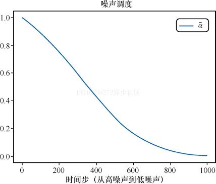
下面是绘制加噪alpha的随时间步的变化：

# 绘制'alpha'，'alpha'（即α）在DDPM论文中被称为'alpha bar'（即α）。# 为了能够清晰地表现出来，我们# 选择使用Diffusers中的alphas_cumprod函数来得到alphas）timesteps = pipe.scheduler.timesteps.cpu()alphas = pipe.scheduler.alphas_cumprod[timesteps]plt.plot(timesteps, alphas, label='alpha_t');plt.legend();

标准DDIM（https://arxiv.org/abs/2010.02502）采样的实现代码如下所示：

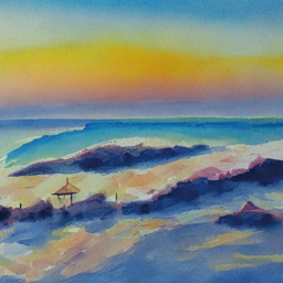
# 采样函数（标准的DDIM采样）@torch.no_grad()def sample(prompt, start_step=0, start_latents=None,           guidance_scale=3.5, num_inference_steps=30,           num_images_per_prompt=1, do_classifier_free_ guidance=True,           negative_prompt='', device=device):# 对文本提示语进行编码    text_embeddings = pipe._encode_prompt(            prompt, device, num_images_per_prompt,             do_classifier_free_guidance, negative_prompt    )# 配置推理的步数    pipe.scheduler.set_timesteps(num_inference_steps, device=device)　# 如果没有起点，就创建一个随机的起点    if start_latents is None:       start_latents = torch.randn(1, 4, 64, 64, device=device)       start_latents *= pipe.scheduler.init_noise_sigma　    latents = start_latents.clone()　    for i in tqdm(range(start_step, num_inference_steps)):            t = pipe.scheduler.timesteps[i]# 如果正在进行CFG，则对隐层进行扩展    latent_model_input = torch.cat([latents] * 2)  if do_classifier_free_guidance else latents    latent_model_input = pipe.scheduler.scale_model_input(latent_       model_input, t)# 预测残留的噪声    noise_pred = pipe.unet(latent_model_input, t, encoder_hidden_       states=text_embeddings).sample# 进行引导    if do_classifier_free_guidance:            noise_pred_uncond, noise_pred_text = noise_pred.chunk(2)            noise_pred = noise_pred_uncond + guidance_scale *                (noise_pred_text - noise_pred_uncond)　    # 使用调度器更新步骤        # latents = pipe.scheduler.step(noise_pred, t, latents). # prev_sample # 现在不用调度器，而是自行实现        prev_t = max(1, t.item() - (1000//num_inference_steps)) # t-1        alpha_t = pipe.scheduler.alphas_cumprod[t.item()]        alpha_t_prev = pipe.scheduler.alphas_cumprod[prev_t]        predicted_x0 = (latents - (1-alpha_t).sqrt()*noise_pred) /            alpha_t.sqrt()        direction_pointing_to_xt = (1-alpha_t_prev).sqrt()*noise_           pred        latents = alpha_t_prev.sqrt()*predicted_x0 + direction_           pointing_to_xt# 后处理　    images = pipe.decode_latents(latents)    images = pipe.numpy_to_pil(images)　    return images# 生成一张图片，测试一下采样函数，效果如图7-4所示sample('Watercolor painting of a beach sunset', negative_prompt=    negative_prompt, num_inference_steps=50)[0].resize((256, 256))

四、DDIM反转

       反转的目标是”颠倒“采样的过程。我们最终想得到”带噪“的隐式表示。如果将其用作采样过程的起点，那么生成的图像将是原始图像。

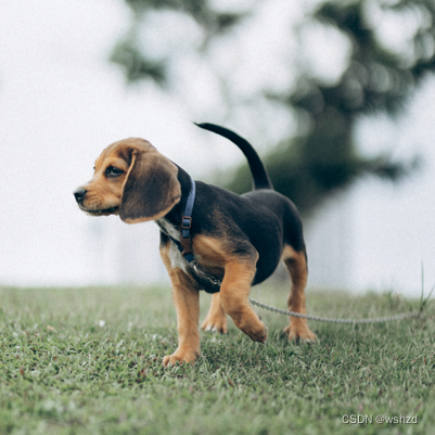
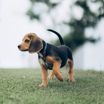
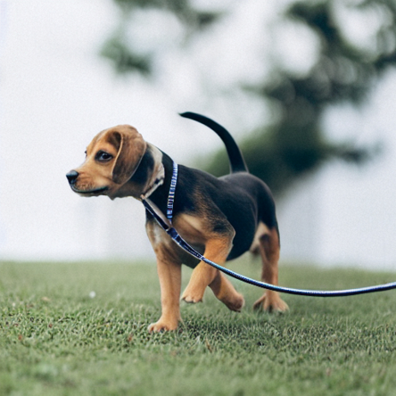
       我们现在首先来加载一张图像，来看看DDIM反转如何做？有什么效果？

#图片来源：https://www.pexels.com/photo/a-beagle-on-green-grass- # field-8306128/（代码中使用对应的JPEG文件链接）input_image = load_image('https://images.pexels.com/photos/ 8306128/pexels-photo-8306128.jpeg', size=(512, 512))

       我们使用一个包含无分类器引导的文本Prompt来进行反转操作，代码如下：

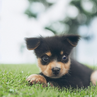
input_image_prompt = "Photograph of a puppy on the grass"

       接下来，我们将这幅PIL图像转换为一系列隐式表示，这些隐式表示将被用作反转操作的起点。

# 使用VAE进行编码with torch.no_grad(): latent = pipe.vae.encode(tfms.functional.to_   tensor(input_image).unsqueeze(0).to(device)*2-1)l = 0.18215 * latent.latent_dist.sample()

       我们使用invert函数进行反转，可以看出invert与上面的sample函数非常类似，但是invert函数是朝相反的方向移动的：从t=0开始，想噪声更多的方向移动的，而不是在更新隐式层的过程中那样噪声越来越少。我们可以利用预测的噪声来撤回一步更新操作，并从t移动到t+1。

## 反转@torch.no_grad()def invert(start_latents, prompt, guidance_scale=3.5,           num_inference_steps=80,num_images_per_prompt=1,            do_classifier_free_guidance=True, negative_prompt='',            device=device): # 对提示文本进行编码    text_embeddings = pipe._encode_prompt(      prompt, device, num_images_per_prompt,      do_classifier_free_guidance, negative_prompt     )     # 已经指定好起点     latents = start_latents.clone()     # 用一个列表保存反转的隐层     intermediate_latents = []     # 配置推理的步数     pipe.scheduler.set_timesteps(num_inference_steps,device=device)      # 反转的时间步     timesteps = reversed(pipe.scheduler.timesteps)　     for i in tqdm(range(1, num_inference_steps), total=num_         inference_steps-1): # 跳过最后一次迭代     if i >= num_inference_steps - 1: continue　     t = timesteps[i] # 如果正在进行CFG，则对隐层进行扩展　     latent_model_input = torch.cat([latents] * 2) if do_        classifier_free_guidance else latents     latent_model_input = pipe.scheduler.scale_model_        input(latent_model_input, t)     # 预测残留的噪声      noise_pred = pipe.unet(latent_model_input, t, encoder_        hidden_states=text_embeddings).sample     # 进行引导     if do_classifier_free_guidance:        noise_pred_uncond, noise_pred_text = noise_pred.chunk(2)        noise_pred = noise_pred_uncond + guidance_scale *        (noise_pred_text - noise_pred_uncond)current_t = max(0, t.item() - (1000//num_inference_steps))#tnext_t = t # min(999, t.item() + (1000//num_inference_steps)) # t+1alpha_t = pipe.scheduler.alphas_cumprod[current_t]alpha_t_next = pipe.scheduler.alphas_cumprod[next_t]　# 反转的更新步（重新排列更新步，利用xt-1（当前隐层）得到xt（新的隐层））latents = (latents - (1-alpha_t).sqrt()*noise_pred)*(alpha_t_next.   sqrt()/alpha_t.sqrt()) + (1-alpha_t_next).sqrt()*noise_pred# 保存intermediate_latents.append(latents)return torch.cat(intermediate_latents)

将invert函数应用于上述小狗的图片，得到图片的一系列隐式表示。

inverted_latents = invert(l, input_image_prompt,num_inference_steps=50)inverted_latents.shape

# 输出torch.Size([48, 4, 64, 64])

将得到的最终隐式表示作为起点噪声，尝试新的采样过程。

# 解码反转的最后一个隐层with torch.no_grad():  im = pipe.decode_latents(inverted_latents[-1].unsqueeze(0))pipe.numpy_to_pil(im)[0]

通过调用call方法将反转隐式表示输入给Pipeline。

pipe(input_image_prompt, latents=inverted_latents[-1][None],      num_inference_steps=50, guidance_scale=3.5).images[0]

      看到生成的图片是不是有点蒙了，这不是刚开始输入的图片呀？

      这是因为DDIM反转需要一个重要的假设-在时刻t预测的噪声与在时刻t+1预测的噪声相同，但这个假设在反转50步或100步是不成立的。

       我们既可以使用更多的时间步来得到更准确的反转，也可以采取”作弊“的方法，直接从相应反转过程50步中的第20步的隐式表示开始。

# 设置起点的原因start_step=20sample(input_image_prompt, start_latents=inverted_latents[-(start_step+1)][None], start_step=start_step, num_inference_steps=50)[0]

      经过这一折腾，生成的图片和原始图片很接近了，那为什么要这么做呢？

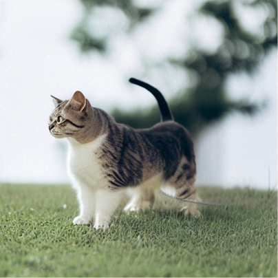
       因为我们现在想用一个新的文本Prompt来生成图片。我们想要得到一张除了与Prompt相关以外，其他内容都与原始图片大致相同的图片。例如，将小狗换成小猫，得到的结果如下所示：

# 使用新的文本提示语进行采样start_step=10new_prompt = input_image_prompt.replace('puppy', 'cat')sample(new_prompt, start_latents=inverted_latents[-(start_step+1)]       [None],start_step=start_step, num_inference_steps=50)[0]

       到此为止，读者可能有一些疑问，比如为什么不直接使用Img2Img？为什么要反转？为什么不直接对输入图像添加噪声，然后用新的Prompt直接”去噪“呢？

       其实是可以采用上述方法做的，但是生成的效果对添加的噪声量十分敏感，噪声量大时会生成十分夸张的图片，噪声量小时生成的图片几乎没有变化。

start_step = 10num_inference_steps=50pipe.scheduler.set_timesteps(num_inference_steps)noisy_l = pipe.scheduler.add_noise(l, torch.randn_like(l), pipe.   scheduler.timesteps[start_step])sample(new_prompt, start_latents=noisy_l, start_step=start_step,     num_inference_steps=num_inference_steps)[0]

五、DDIM反转整体方案

      将上述代码封装到一个简单函数中，并输入一张图片和两个文本Prompt，便可以得到一张通过反转修改后的图片。

def edit(input_image, input_image_prompt, edit_prompt, num_steps=100, start_step=30,guidance_scale=3.5):    with torch.no_grad(): latent = pipe.vae.encode(tfms.functional.      to_tensor(input_image).unsqueeze(0).to(device)*2-1)    l = 0.18215 * latent.latent_dist.sample()    inverted_latents = invert(l, input_image_prompt,num_inference_       steps=num_steps)    final_im = sample(edit_prompt, start_latents=inverted_latents[       -(start_step+1)][None],start_step=start_step, num_inference_       steps=num_steps,guidance_scale=guidance_scale)[0]    return final_imAnd in action: # 实际操作edit(input_image, 'A puppy on the grass', 'an old grey dog on  the grass', num_steps=50,start_step=10) 

修改一下Prompt和参数来看看效果如何不同

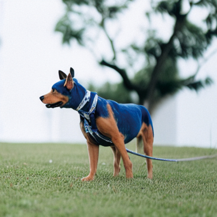
edit(input_image, 'A puppy on the grass', 'A blue dog on the lawn',  num_steps=50,start_step=12, guidance_scale=6) 

得到如下图片

更多迭代能够得到更好的表现，我们可以测试一下

# 更多步的反转测试edit(input_image, 'A puppy on the grass', 'A puppy on the grass',     num_steps=350, start_step=1)

我们换一张图片进行测试一下看看效果

原始图片如下所示：

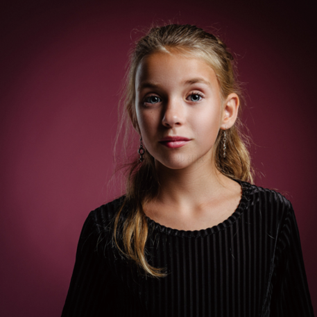
# 图片来源：https://www.pexels.com/photo/girl-taking-photo-1493111/ # （代码中使用对应的JPEG文件链接）face = load_image('https://images.pexels.com/photos/1493111/pexels- photo-1493111.jpeg', size=(512, 512))

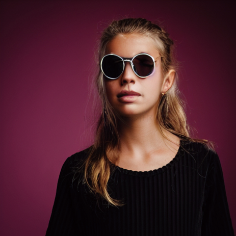
edit(face, 'A photograph of a face', 'A photograph of a face with sunglasses', num_steps=250, start_step=30, guidance_scale=3.5)

生成的效果如下所示：

PS：读者可以通过测试不同的Prompt来观察生成的效果，强烈建议了解一下Null-text Inversion：一个基于DDIM来优化空文本（无条件Prompt）的反转过程，有更准确的反转过程与更好的编辑效果。