国科大机器人作业五：EKF SLAM (实验部分)

第五次机器人作业：EKF Simultaneous Localization And Mapping (SLAM)

1 Introduction

本次练习建立在练习4的基础上，不同的是，基于地标定位的练习4依赖先验地图，而本次练习在探索环境的时候，自主建立地图。

2 EKF SLAM

EKF SLAM 用概率的方法去估计地图和机器人位姿，所以要添加一些地标的参数去表示EKF状态

这里我们假设地标是静态的，地标表示在一个状态向量中，地标之间的相关性和不确定性均已知。其数量和启动之前的估计也已知。

2.1 Time Update (propagation)

Task：任务

• 再利用练习4的结果，去推导和实现上面定义状态的状态预测和协方差传播
• 最后，修改transitionFunction.m状态转移函数，

Validation：验证

• 运行test/validateTransitionFunction.m函数
• 如果正确，得到输出State transition function appears to be correct!.

插入代码

function [f, F_x, F_u] = transitionFunction(x,u,b)
% [f, F_x, F_u] = transitionFunction(x,u,b) predicts the state x at time t given
% the state at time t-1 and the input u at time t. b is the distance between
% the wheels f the differential-drive robot. F_x denotes the Jacobian
% of the state transition function with respect to the state evaluated at
% the state and input provided. F_u denotes the Jacobian of the state
% transition function with respect to the input evaluated at the state and
% input provided.
% State and input are defined according to the book pp. 337

if nargin < 3 || isempty(b)
    b = .1;
end

del_s = (u(2) + u(1))/2;
del_t = (u(2) - u(1))/b;

f = x(:);
f(1:3,1) = [x(1); x(2); x(3)] + [del_s*cos(x(3)+del_t/2); del_s*sin(x(3)+del_t/2); del_t];


F_x = eye(size(x,1));
F_x(1,3) = -del_s*sin(x(3)+del_t/2); 
F_x(2,3) = del_s*cos(x(3) + del_t/2); 

F_u = zeros(size(x,1),2);
F_u(1:3,1:2) = [0.5*cos(x(3)+del_t/2)+(del_s/(2*b))*sin(x(3)+del_t/2), 0.5*cos(x(3)+del_t/2)-(del_s/(2*b))*sin(x(3)+del_t/2); ...
       0.5*sin(x(3)+del_t/2)-(del_s/(2*b))*cos(x(3)+del_t/2), 0.5*sin(x(3)+del_t/2)+(del_s/(2*b))*cos(x(3)+del_t/2); ...
       -1/b 1/b];

运行validateTransitionFunction.m验证

>> validateTransitionFunction
State transition function appears to be correct!

2.2 Measurement Update

Task：任务

• 修改measurementFunction.m.函数
• 实现一个测量函数，该函数返回给定的状态矢量（现在包括机器人状态和地标）和等式6中定义的地标索引的预测测量
• 另外，提供相对于状态向量的测量的对应雅可比行列式。与练习4相比，界标位置现在是状态向量的一部分。这必须反映在雅可比算术中

Validation：验证

• 运行test/validateMeasurementFunction.m函数

插入代码

function [h, H_x] = measurementFunction(x, idxLandmark)
% [h, H_x] = measurementFunction(x, idxLandmark) returns the predicted measurement
% given a state x and a single map entry with index idxLandmark. H_x denotes the Jacobian of the
% measurement function with respect to the state evaluated at the state
% provided.
% Map entry and state are defined according to the book pp. 337-338

%Extract individual landmark from the state vector
m = x(3+2*(idxLandmark-1)+1:3+2*(idxLandmark));

if x(1,1) == 0 || x(2,1) == 0 
    h = [0;0];
    H_x = zeros(2,length(x));
    return
end

h  = [m(1) - x(3); m(2) - (x(1,1)*cos(m(1))+x(2,1)*sin(m(1)))];

H_x = zeros(2,length(x));

H_x(1:2,1:3) = [0 0 -1; -cos(m(1)) -sin(m(1)) 0];

%Do not correct first two landmarks as they remain fixed
if (idxLandmark>2)

   H_x(1,3 + (idxLandmark-1)*2+1) = 1;
   H_x(2,3 + (idxLandmark-1)*2+1) =  x(1)*sin(m(1))-x(2)*cos(m(1));
   H_x(1,3 + (idxLandmark)*2) = 0;
   H_x(2,3 + (idxLandmark)*2) = 1;
end

[h(1), h(2), isRNegated] = normalizeLineParameters(h(1), h(2));

if isRNegated 
    H_x(2, :) = - H_x(2, :);
end

运行validateMeasurementFunction.m函数（将help_函数都包含上，省的排查）

>> validateMeasurementFunction
measurement function appears to be correct!

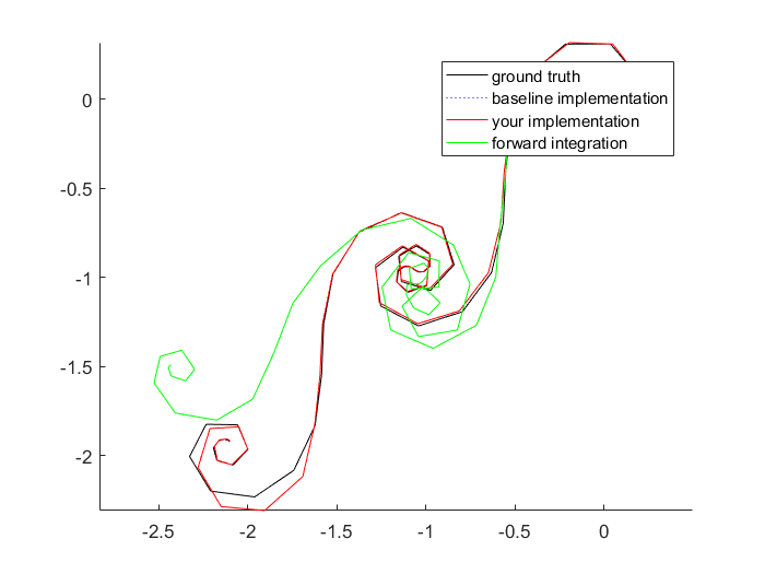
2.3 Validation of Complete EKF SLAM System

随着状态传播和测量更新的进行，现在是时候验证完整的EKF SLAM设置了。

• 运行test/validateFilter.m.函数，这将评估过滤器是否将提供与基准实施相同的输出

>> validateFilter
State transition function appears to be correct!

• 运行test/validateCompleteEKFLoop.m函数，使用随机生成的输入值评估过滤器

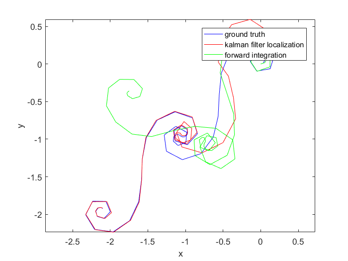
可见CompleteEKF算法的跟踪精度非常精确

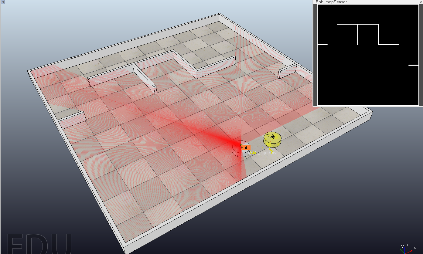
3 V-REP Experiment

Task：任务

至此，EKF localization and mapping都已经通过0测试，接下来在VREP中测试一下整体功能

Validation：验证

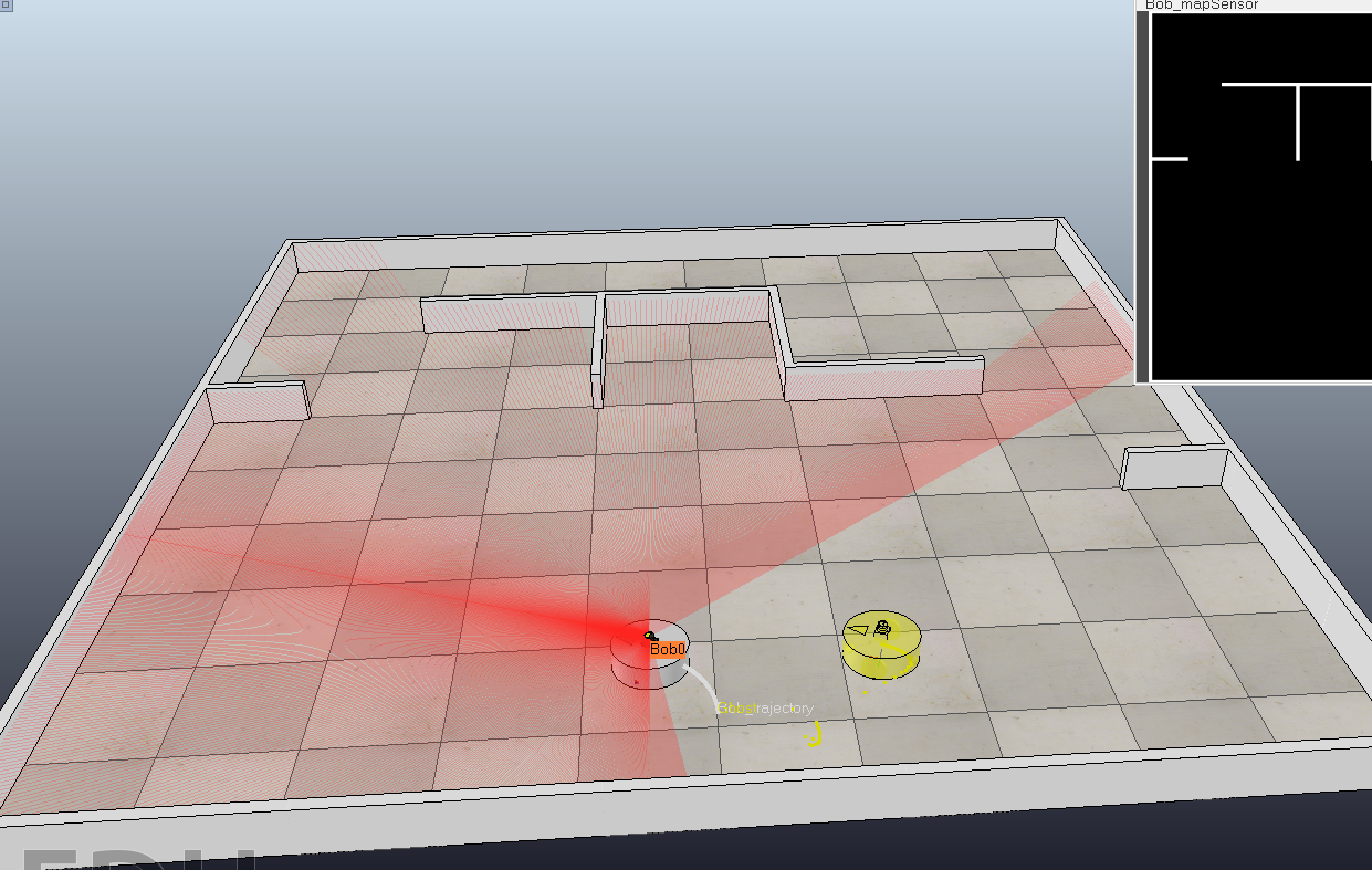
• Start V-REP, load scene scene/mooc_exercises.ttt，运行仿真
• 打开matlab，运行vrep/vrepSimulation.m
• 在实际的机器人旁边，会看到一个黄色的“鬼影”，该图形可以根据本地化情况估算出姿势。如果一切操作正确，将在机器人的姿势之后看到黄色的鬼影