


一、简介
1、对特征选择的指标提供计算方法和代码,包括有:相关系数、互信息、KS、IV、L1正则化、单特征模型评分、特征重要度或系数大小、boruta特征评价、递归特征消除排序。
2、提供特征选择的方法和代码:前向搜索法、遗传算法启发式搜索法,最佳特征检测法,
# 本次项目使用的数据为以下数据,
from sklearn.datasets import load_breast_cancer
data = load_breast_cancer()
data['data'].shape
X,y= data['data'],data.target

# 模型使用的逻辑回归,评价指标为auc值,使用代码为封装的Feature_select类,代码附后
from tools.feature_select import Feature_select
fs = Feature_select(X,y,lr)
二、特征选择指标
1.皮尔森相关系数
Pearson相关系数反应了特征和标签之间的线性关系,其一个明显缺陷是,作为特征排序机制,他只对线性关系敏感。如果关系是非线性的,即便两个变量具有一一对应的关系,Pearson相关性也可能会接近0。
fs.corr()
array([-0.73002851, -0.4151853 , -0.74263553, -0.70898384, -0.35855997,
       -0.59653368, -0.69635971, -0.77661384, -0.33049855,  0.0128376 ,
       -0.56713382,  0.00830333, -0.5561407 , -0.54823594,  0.06701601,
       -0.29299924, -0.25372977, -0.40804233,  0.00652176, -0.07797242,
       -0.77645378, -0.45690282, -0.78291414, -0.73382503, -0.42146486,
       -0.59099824, -0.65961021, -0.79356602, -0.41629431, -0.32387219])
2.互信息
相比皮尔森相关系数 ,互信息能够一定程度反应特征和标签之间的非线性关系。
fs.mic()
array([0.36671567, 0.09648092, 0.40428514, 0.35976973, 0.08173721,
       0.21061423, 0.37479754, 0.44305847, 0.06671437, 0.01354967,
       0.24521911, 0.00110187, 0.278233  , 0.33920662, 0.01602095,
       0.07457715, 0.11807899, 0.12371226, 0.013367  , 0.04097258,
       0.44985384, 0.12364186, 0.47728208, 0.46426447, 0.10166035,
       0.22460362, 0.31435137, 0.43651194, 0.09544855, 0.06837461])
3.KS和IV值
KS和IV值作为风控中经常使用的两个指标,IV值更加注重特征对标签的区分能力,KS值注重模型对于标签的区分
fs.ks_iv()
(array([0.72390466, 0.45248666, 0.74467523, 0.73142276, 0.31537709,
        0.57175889, 0.75971143, 0.81985624, 0.30314201, 0.05657735,
        0.6018313 , 0.08626658, 0.5867951 , 0.70708472, 0.02433804,
        0.37730564, 0.48077533, 0.45248666, 0.00573437, 0.2043893 ,
        0.79730194, 0.44318482, 0.82737435, 0.80482004, 0.40636066,
        0.54920459, 0.70058401, 0.80290418, 0.33869774, 0.29537287]),
 array([3.78395724, 1.5824873 , 3.82087721, 3.82234285, 1.34695804,
        2.10298612, 3.00830869, 3.9745556 , 1.31276152, 1.15309762,
        2.53434592, 1.06847433, 2.80319049, 3.65151974, 1.06348267,
        1.39990837, 1.61294779, 1.59034111, 1.06672724, 1.14612131,
        4.44837968, 1.54256612, 4.58499352, 4.39469498, 1.48978388,
        2.19735313, 2.57167549, 4.37557075, 1.63321251, 1.33836142]))
4.L1正则化
L1正则化将系数w的l1范数作为惩罚项加到损失函数上,由于正则项非零,这就迫使那些弱的特征所对应的系数变成0。因此L1正则化往往会使学到的模型很稀疏(系数w经常为0),这个特性使得L1正则化成为一种很好的特征选择方法。
这里采用sklearn总lasso模型进行封装
fs.l1_select(alpha=0.01) # alpha 系数越大,系数为0的特征越多
array([ 0.        ,  0.00202185,  0.        ,  0.00043358, -0.        ,
       -0.        , -0.        , -0.        , -0.        , -0.        ,
       -0.        , -0.        , -0.        , -0.00125443, -0.        ,
       -0.        , -0.        , -0.        , -0.        , -0.        ,
       -0.08225553, -0.01460497, -0.01379535,  0.0007448 , -0.        ,
       -0.        , -0.06013473, -0.        , -0.        , -0.        ])
5.基于学习模型的特征评分
这种方法的思路是直接使用你要用的机器学习算法,针对每个单独的特征和响应变量建立预测模型,得出模型的评分。
其实Pearson相关系数等价于线性回归里的标准化回归系数。假如某个特征和响应变量之间的关系是非线性的,可以用基于树的方法(决策树、随机森林)、或者扩展的线性模型等。基于树的方法比较易于使用,因为他们对非线性关系的建模比较好,并且不需要太多的调试。但要注意过拟合问题,因此树的深度最好不要太大,再就是运用交叉验证。
fs.learn()
array([0.94065577, 0.77690815, 0.94993828, 0.9414743 , 0.72440823,
       0.86654102, 0.93679947, 0.96337183, 0.70027988, 0.46412392,
       0.86841319, 0.46160936, 0.87624184, 0.92835235, 0.5316104 ,
       0.72631256, 0.7815463 , 0.79461106, 0.46528705, 0.6198184 ,
       0.97066582, 0.78313947, 0.97697965, 0.97057468, 0.75707131,
       0.86194584, 0.92023563, 0.96808801, 0.73623915, 0.68791135])
6.特征重要程度或系数大小(select_from_model)
封装sklearn中Select_from_model,不过这个方法只能输出选择之后的特征,不能输出具体的评价分数,分析select_from_model代码,针对随机森林等模型,则输入其feature_important_大小。如回归模型,则输出其系数的大小。
fs.select_from_model()
array([0.66640051, 0.30333585, 0.36057931, 0.01055394, 0.02294638,
       0.11137151, 0.15632322, 0.06555693, 0.03189341, 0.00623842,
       0.02738789, 0.24660799, 0.06654065, 0.12058007, 0.00211526,
       0.02430511, 0.03371127, 0.00860147, 0.00775326, 0.00222996,
       0.7054829 , 0.37988099, 0.24474795, 0.01677032, 0.04206173,
       0.35002252, 0.43570279, 0.12673618, 0.10253126, 0.03317253])
7.boruta特征选择
boruta的思路是针对某一特征,将其值进行随机分配,形成该特征的shadow特征,通过比较原始特征和shadow特征的重要对差异,判断该特征的有效性。这一方法的优点是,形成了对照组,提出了部分不能观察到的因素造成对特征评分的误判。
fs.boruta()
[ 1.93884227e-02  2.55134195e-02 -2.22229096e-02  9.71757303e-04
  3.42173146e-04  4.67893675e-03  6.91337507e-03  2.69658857e-03
  4.77232016e-04 -2.64284804e-04 -2.54539319e-04 -2.34624522e-03
  3.69165467e-03  3.24437344e-02  3.30642361e-05  1.05415307e-03
  1.47101778e-03  3.76387825e-04  1.92383814e-04  8.18088312e-05
  2.77834702e-02  1.12243313e-01 -1.26686099e-02  2.19071929e-02
  1.22108470e-03  1.62224294e-02  2.05164881e-02  5.65378210e-03
  4.06231930e-03  1.34338174e-03]
8.递归特征消除
递归特征消除的主要思想是反复的构建模型(如SVM或者回归模型)然后选出最好的(或者最差的)的特征(可以根据系数来选),把选出来的特征放到一遍,然后在剩余的特征上重复这个过程,直到所有特征都遍历了。这个过程中特征被消除的次序就是特征的排序。因此,这是一种寻找最优特征子集的贪心算法。
Sklearn提供了RFE包,可以用于特征消除,还提供了RFECV,可以通过交叉验证来对的特征进行排序。这里 封装sklearn中的RFECV,将得分排名反转,得到评分。
fs.rfecv()
[13  9  5  2 10 13 13 13 12  3 13 13 13 13  0 13  8  6  4  1 11 13 13  7
 13 13 13 13 13 13]
9.全部指标计算和综合评价
# 计算以上全部指标,并完成归一化之后,按照分配的权重计算综合得分(score),并按照得分进行排序
fs.feature_eval(eval_weight=[0.1, 0.1, 0.1, 0.1, 0.1, 0.2, 0.2, 0.2, 0.2])
	corr		mic      	ks      	iv			l1			learn		bourta		important	rfecv		score
22	-0.782914	0.474132	0.827374	4.584994	-0.018573	0.976980	0.009898	0.244748	13.0	100.000000
20	-0.776454	0.453242	0.797302	4.448380	-0.000000	0.970666	0.034960	0.705483	11.0	94.078947
0	-0.730029	0.365405	0.723905	3.783957	-0.000000	0.940656	0.024852	0.666401	13.0	88.815789
27	-0.793566	0.436879	0.802904	4.375571	-0.000000	0.968088	0.006664	0.126736	13.0	86.842105
13	-0.548236	0.340502	0.707085	3.651520	-0.000056	0.928352	0.032520	0.120580	13.0	81.907895
26	-0.659610	0.317450	0.700584	2.571675	-0.000000	0.920236	0.023289	0.435703	13.0	81.578947
7	-0.776614	0.439923	0.819856	3.974556	-0.000000	0.963372	0.003340	0.065557	13.0	80.921053
6	-0.696360	0.373305	0.759711	3.008309	-0.000000	0.936799	0.008183	0.156323	13.0	78.947368
2	-0.742636	0.401514	0.744675	3.820877	-0.000000	0.949938	-0.021761	0.360579	5.0		78.618421
23	-0.733825	0.464017	0.804820	4.394695	0.000316	0.970575	0.021532	0.016770	7.0		77.302632
21	-0.456903	0.117602	0.443185	1.542566	-0.009721	0.783139	0.118309	0.379881	13.0	75.657895
25	-0.590998	0.226403	0.549205	2.197353	-0.000000	0.861946	0.018325	0.350023	13.0	71.381579
5	-0.596534	0.212811	0.571759	2.102986	-0.000000	0.866541	0.005434	0.111372	13.0	64.802632
12	-0.556141	0.276573	0.586795	2.803190	-0.000000	0.876242	0.001964	0.066541	13.0	63.157895
3	-0.708984	0.358486	0.731423	3.822343	0.000289	0.941474	0.001050	0.010554	2.0		54.934211
10	-0.567134	0.246681	0.601831	2.534346	-0.000000	0.868413	-0.000403	0.027388	13.0	52.960526
28	-0.416294	0.089774	0.338698	1.633213	-0.000000	0.736239	0.004665	0.102531	13.0	51.644737
1	-0.415185	0.090539	0.452487	1.582487	-0.000000	0.776908	0.002043	0.303336	9.0		48.190789
24	-0.421465	0.097283	0.406361	1.489784	-0.000000	0.757071	0.001480	0.042062	13.0	45.723684
16	-0.253730	0.116072	0.480775	1.612948	-0.000000	0.781546	0.001675	0.033711	8.0		39.473684
15	-0.292999	0.073890	0.377306	1.399908	-0.000000	0.726313	0.001138	0.024305	13.0	36.184211
11	0.008303	0.000000	0.086267	1.068474	-0.000000	0.461609	-0.002358	0.246608	13.0	36.184211
29	-0.323872	0.068337	0.295373	1.338361	-0.000000	0.687911	0.001587	0.033173	13.0	35.526316
17	-0.408042	0.128856	0.452487	1.590341	-0.000000	0.794611	0.000476	0.008601	6.0		32.401316
8	-0.330499	0.065021	0.303142	1.312762	-0.000000	0.700280	0.000441	0.031893	12.0	26.315789
4	-0.358560	0.078689	0.315377	1.346958	-0.000000	0.724408	0.000347	0.022946	10.0	24.671053
19	-0.077972	0.039776	0.204389	1.146121	-0.000000	0.619818	0.000093	0.002230	1.0		5.592105
9	0.012838	0.008280	0.056577	1.153098	-0.000000	0.464124	-0.000292	0.006238	3.0		4.934211
18	0.006522	0.015024	0.005734	1.066727	-0.000000	0.465287	0.000227	0.007753	4.0		4.605263
14	0.067016	0.014678	0.024338	1.063483	-0.000000	0.531610	0.000052	0.002115	0.0		0.000000
三、特征选择方法
以上各种指标为特征选择提供参考,下面提供特征选择的方法,可以直接获得较为优化的特征组合
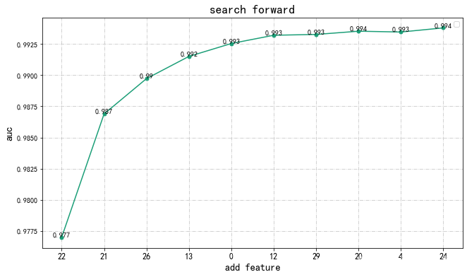
1.前向搜索
从第一个特征开始选取最优的特征放入特征组合列表中,然后组合第一个选取的特征和其他特征,同样选择评分最佳的组合,将这两个放入特征组合列表中,以此类推,直至数量满足要求。
sf = fs. search_forward(max_feature = 10) #设定向前搜索的最大特征数量,
0 select [22],  	the score :0.976979653545736
1 select [22, 21],  	the score :0.9868864998778198
2 select [22, 21, 26],  	the score :0.9897221832285703
3 select [22, 21, 26, 13],  	the score :0.9915044314118994
4 select [22, 21, 26, 13, 0],  	the score :0.992541012656473
5 select [22, 21, 26, 13, 0, 12],  	the score :0.993202973222626
6 select [22, 21, 26, 13, 0, 12, 29],  	the score :0.9932691107887637
7 select [22, 21, 26, 13, 0, 12, 29, 20],  	the score :0.9935280286369379
8 select [22, 21, 26, 13, 0, 12, 29, 20, 4],  	the score :0.9934640790479309
9 select [22, 21, 26, 13, 0, 12, 29, 20, 4, 24],  	the score :0.9937947668786189
2.遗传算法启发式
通过启发式算法,在所有特征组合空间,寻找最优特征组合,实现模型评分最大值。时间消耗很大,且具有随机性,可以通过设定初始族群完成
# 使用遗传算法进行特征选择,迭代100次,最大特征限制为10
ga = fs.selcet_by_GA(it_num=100,max_feature=10,mutation=0.4)  #
0/100,	当前分数:0.9920092042348839
1/100,	当前分数:0.9920092042348839
2/100,	当前分数:0.9920092042348839
3/100,	当前分数:0.9920092042348839
4/100,	当前分数:0.9920278778614842
5/100,	当前分数:0.9930635275910416
6/100,	当前分数:0.9930635275910416
7/100,	当前分数:0.9930635275910416
8/100,	当前分数:0.9930635275910416
9/100,	当前分数:0.9930635275910416
10/100,	当前分数:0.9930635275910416
11/100,	当前分数:0.9930635275910416
12/100,	当前分数:0.9930635275910416
13/100,	当前分数:0.9930635275910416
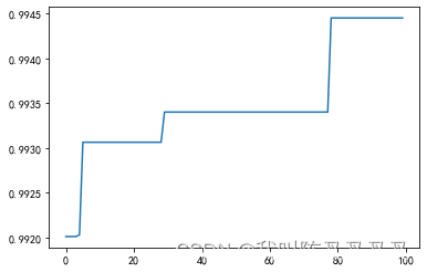
# 遗传算法最优的特征组合
ga[1]
[0, 2, 13, 15, 17, 19, 21, 23, 24, 26]
遗传算法解0.9944533479949463 ,大于前向搜索
3.最优特征检测
使用其他特征以此替换特征组合中的特征,如发现更优解则进行替换,如没有则保留,返回结果
fs.test_best([0, 2, 13, 15, 17, 19, 21, 23, 24, 26])
loc0 is done
loc1 is done
loc2 is done
the col 15 ,	loc3 is replaceed by 6
loc3 is done
the col 17 ,	loc4 is replaceed by 15
the col 17 ,	loc4 is replaceed by 28
loc4 is done
loc5 is done
loc6 is done
loc7 is done
loc8 is done
loc9 is done
([0, 2, 13, 6, 28, 19, 21, 23, 24, 26], 0.9945843666651069)
通过最优组合检验之后 发现更优解评分为0.9945 大于之前遗传算法找到的最优解
四、特征选择封装代码
import  pandas as pd
import  numpy as np
from sklearn.model_selection import cross_val_score

class Feature_select:
    def __init__(self, X, y,model,scoring='roc_auc'):
        '''
        X:np.array,features
        y:np.array,label
        '''
        self.X = X
        self.y = y
        self.model = model
        self.scoring = scoring
    def corr(self):
        '''
        关系数计算:输出每一个特征对应的相关系数
        '''
        corr_ = pd.DataFrame(np.hstack([self.X, self.y.reshape(-1, 1)])).corr().iloc[:-1, -1]
        corr_ = np.array(corr_)
        return corr_

    def mic(self):
        '''
        mic系数计算:输出每一个特征对应的mic值
        '''
        from sklearn.feature_selection import mutual_info_classif as mic
        mic_ = mic(self.X, self.y)
        return mic_

    def ks_iv(self):
        '''
        ks和iv计算函数
        '''
        iv_, ks_ = [], []
        for i in range(self.X.shape[1]):
            cuted = pd.qcut(self.X[:, i], q=10, labels=False)
            num_table = pd.crosstab(cuted, self.y)
            good_sum = num_table.sum()[0]
            bad_sum = num_table.sum()[1]
            iv = (((num_table.iloc[:, 1] + 0.5) / bad_sum) - ((num_table.iloc[:, 0] + 0.5) / good_sum) * np.log(
                ((num_table.iloc[:, 1] + 0.5) / bad_sum) / ((num_table.iloc[:, 0] + 0.5) / good_sum))).sum()
            iv_.append(iv)
            ks = max((num_table.iloc[:, 1] / bad_sum).cumsum() - (num_table.iloc[:, 0] / good_sum).cumsum())
            ks_.append(ks)
        return np.array(ks_), np.array(iv_)

    def l1_select(self, alpha=0.15):
        '''
        L1正则化 返回为0的为被剔除变量
        alpha:惩罚系数大小
        '''
        from sklearn.linear_model import Lasso
        lasso = Lasso(alpha=alpha)  # alpha 系数越大 选出的0就越多
        lasso.fit(self.X, self.y)
        return lasso.coef_

    def learn(self):
        '''
        单个特征进入模型时候的五折交叉验证评价指标
        model:评价模型
        scoring:评价指标
        (每个特征需运行一次模型,时间较长)
        '''
        scores = []
        for i in range(self.X.shape[1]):
            score = cross_val_score(self.model, self.X[:, i].reshape(-1, 1), self.y, scoring=self.scoring, cv=5)
            scores.append(np.mean(score))
        return np.array(scores)

    def select_from_model(self):
        '''
        sklean 中select_from_model
        model:训练模型
            针对部分树模型:返回其特征重要度,
            针对线性模型:返回其系数绝对值
        '''
        from sklearn.feature_selection import SelectFromModel
        s_model = SelectFromModel(self.model).fit(self.X, self.y)
        try:
            important_ = s_model.estimator_.feature_importances_
        except:
            important_ = abs(s_model.estimator_.coef_[0])
        return important_

    def boruta(self, it_num=40):
        '''
        参照Boruta思想,通过打乱之前特征的数值,构建shadow特征,比较原始特征和shadow特征的重要程度,评价特征的有效性
        :param it_num: int,迭代次数
        :return: 特征的Boruta得分
        '''
        diff_record = []
        for i in range(it_num):
            X_shadow = self.X.copy()
            np.random.shuffle(X_shadow)
            X_boruta = np.hstack([self.X, X_shadow])
            import_ = Feature_select(X_boruta, self.y, self.model).select_from_model()
            import_ = import_.reshape((2, -1))
            diff_ = import_[0, :] - import_[1, :]
            diff_record.append(diff_)
        bouruta_score = pd.DataFrame(np.array(diff_record).T).mean(1)
        return np.array(bouruta_score)

    def rfecv(self):
        '''
        封装sklearn中的RFECV,将得分排名反转,得到评分
        :return:
        '''
        from sklearn.feature_selection import RFECV
        w = RFECV(self.model, scoring=self.scoring).fit(self.X, self.y)
        return w.ranking_.max() - w.ranking_

    def search_forward(self, max_feature):
        '''
        从第一个特征开始选取最优的特征放入特征组合列表中,然后组合第一个选取的特征和其他特征,同样选择评分最佳的组合,将这两个放入特征组合列表中,以此类推,直至数量满足要求。
        model:评价模型
        max_feature:需要的最大特征数量
        scoring:选择评分
        '''
        best_cols = []  # 存储最优的特征组合编号
        best_scores = []  # 存储最优特征组合下的得分
        for i in range(max_feature):
            best_score = 0
            for col in range(self.X.shape[1]):
                if col not in best_cols:
                    col_test = best_cols.copy()
                    col_test += [col]
                    if len(col_test) == 1:
                        score = cross_val_score(self.model, self.X[:, col_test].reshape(-1, 1), self.y, scoring=self.scoring).mean()
                    else:
                        score = cross_val_score(self.model, self.X[:, col_test], self.y, scoring=self.scoring).mean()
                    if score > best_score:
                        best_col = col
                        best_score = score
            best_cols += [best_col]
            best_scores.append(best_score)
            print(f'{i} select {best_cols},  \tthe score :{best_score}')
        return best_cols, best_scores

    def selcet_by_GA(self, num_=50, pop=None, it_num=50, inherit=0.8, mutation=0.2, max_feature=None,
                     want_max=True):
        '''
        使用遗传算法选择特征组合实现模型的评分最大
        model:评价使用的模型
        num_:遗传算法族群数量
        pop:初始族群
        it_num:种群的数量
        inherit:种群进行杂交的概率
        mutation:种群进行变异的概率
        max_feature:最大特征数量
        scoring:模型评分
        want_max:求解最大值
        返回值:传入长度为特征数量的0,1向量
                历史种群达到的最优值
        '''

        def fun_(x):
            '''传入长度为特征数量的0,1向量,转化为bool之后作为特征的索引,提取特征子集,使用特征子集进行选了返回目标函数值'''
            feature_no = [i for i, j in enumerate(x) if j == 1]
            X_ = self.X[:, feature_no]
            score = cross_val_score(self.model, X_, self.y, scoring=self.scoring, cv=5).mean()
            if max_feature is not None:
                if len(feature_no) <= max_feature:
                    val = score
                else:
                    val = score / (len(feature_no) * len(feature_no))
            else:
                val = score
            return val if want_max else -val

        len_ = self.X.shape[1]

        if pop is None:
            if max_feature is not None:
                pop = np.random.choice([0, 1], (num_, len_), p=[1 - max_feature / len_, max_feature / len_])
            else:
                pop = np.random.randint(0, 2, (num_, len_))
        best_f = 0
        list_best_f = []
        for _ in range(it_num):
            scores = [fun_(i) for i in pop]
            best_fit_ = scores[np.argmax(scores)]
            if best_fit_ > best_f:
                best_f = best_fit_
                best_p = pop[np.argmax(scores)]
            list_best_f.append(best_f)
            fitness = scores - min(scores) + 0.01
            idx = np.random.choice(np.arange(num_), size=num_, replace=True,
                                   p=(fitness) / (fitness.sum()))
            pop = np.array(pop)[idx]
            new_pop = []
            for father in pop:
                child = father
                if np.random.rand() < inherit:
                    mother_id = np.random.randint(num_)
                    low_point = np.random.randint(len_)
                    high_point = np.random.randint(low_point + 1, len_ + 1)
                    child[low_point:high_point] = pop[mother_id][low_point:high_point]
                    if np.random.rand() < mutation:
                        mutate_point = np.random.randint(0, len_)
                        child[mutate_point] = 1 - child[mutate_point]
                new_pop.append(child)
            pop = new_pop
            print(f'{_}/{it_num},\t当前分数:{best_f}')
        return best_p, list_best_f

    def feature_eval(self,eval_weight = [0.1,0.1,0.1,0.1,0.1,0.2,0.2,0.2,0.2]):
        '''
        特征综合评价函数
        :param eval_weight:list,计算评分时候各项指标的平价权重,默认为'corr','mic','ks','iv','l1','learn','bourta','important'的权重为 [0.1,0.1,0.1,0.1,0.1,0.2,0.2,0.2]
        :return: table_eval 各项指标数据的明细,和综合得分
        '''
        corr_ = self.corr()
        mic_ = self.mic()
        ks_iv_ = self.ks_iv()
        l1_ = self.l1_select()
        learn_ = self.learn()
        bourta_ = self.boruta()
        important_ = self.select_from_model()
        rfecv_ = self.rfecv()
        table_eval = pd.DataFrame(np.array([corr_,mic_,ks_iv_[0],ks_iv_[1],l1_,learn_,bourta_,important_,rfecv_]).T,columns=['corr','mic','ks','iv','l1','learn','bourta','important','rfecv'])
        eval_ = (table_eval.abs().rank() * np.array(eval_weight) / np.array(eval_weight).sum()).sum(1)
        score = 100*(eval_ - eval_.min())/(eval_.max() - eval_.min())
        table_eval['score'] = score
        return  table_eval.sort_values(by = 'score',ascending=False)

    def check_best(self,feature_no):
        '''
        使用其他特征以此替换特征组合中的特征,如发现更优解则进行替换,如没有则保留,返回结果
        :param feature_no:待检验特征
        :return: 检验之后的特征,最新得分
        '''
        best_score = cross_val_score(self.model, self.X[:,feature_no], self.y, scoring=self.scoring, cv=5).mean()
        for i,no in enumerate(feature_no):
            feature_no_t = feature_no.copy()
            for j in range(self.X.shape[1]):
                if j not in feature_no:
                    feature_no_t[i] = j
                    score = cross_val_score(self.model, self.X[:,feature_no_t], self.y, scoring=self.scoring, cv=5).mean()
                    if score > best_score:
                        best_score = score
                        feature_no[i]  = j
                        print(f'the col {no} ,\tloc{i} is replaceed by {j}')
            print(f'loc{i} is done ')
        return  feature_no,best_score


 1605
1605


 被折叠的 条评论
为什么被折叠?
被折叠的 条评论
为什么被折叠?
 到【灌水乐园】发言


