


模型训练两种方式
1 model.fit()
keras的model.fit(0方式:
https://blog.csdn.net/wuruivv/article/details/109372708
#第一步,import
import tensorflow as tf #导入模块
from sklearn import datasets #从sklearn中导入数据集
import numpy as np #导入科学计算模块
import keras

#第二步,train, test
x_train = datasets.load_iris().data #导入iris数据集的输入

y_train = datasets.load_iris().target #导入iris数据集的标签

np.random.seed(120) #设置随机种子,让每次结果都一样,方便对照

np.random.shuffle(x_train) #使用shuffle()方法,让输入x_train乱序

np.random.seed(120) #设置随机种子,让每次结果都一样,方便对照

np.random.shuffle(y_train) #使用shuffle()方法,让输入y_train乱序

tf.random.set_seed(120) #让tensorflow中的种子数设置为120

#第三步,models.Sequential()
model = tf.keras.models.Sequential([ #使用models.Sequential()来搭建神经网络
    tf.keras.layers.Dense(3, activation = "softmax", kernel_regularizer = tf.keras.regularizers.l2()) #全连接层,三个神经元,激活函数为softmax,使用l2正则化
])

#第四步,model.compile()
model.compile(  #使用model.compile()方法来配置训练方法
    optimizer = tf.keras.optimizers.SGD(lr = 0.1), #使用SGD优化器,学习率为0.1
    loss = tf.keras.losses.SparseCategoricalCrossentropy(from_logits = False), #配置损失函数
    metrics = ['sparse_categorical_accuracy'] #标注网络评价指标
)

#第五步,model.fit()
model.fit(  #使用model.fit()方法来执行训练过程,
    x_train, y_train, #告知训练集的输入以及标签,
    batch_size = 32, #每一批batch的大小为32,
    epochs = 500, #迭代次数epochs为500
    validation_split = 0.2, #从测试集中划分80%给训练集
    validation_freq = 20 #测试的间隔次数为20
)

#第六步,model.summary()
model.summary() #打印神经网络结构,统计参数数目
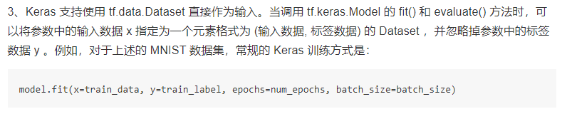
1.1 设置batch_size两种方式
(1)常规的设置,数据集没有设置批次量
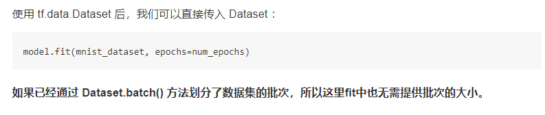
(2)使用了 tf.data.Dataset提前设置了批次量
# 合成了dataset
mnist_dataset = tf.data.Dataset.from_tensor_slices((train_data, train_label))
 获取批次数据
mnist_dataset = mnist_dataset.batch(4)
# 或者
mnist_dataset = mnist_dataset.shuffle(buffer_size=10000).batch(4)
1.2 validation验证集3种方式
1.2.1 从测试集划分20%
本文上面的案例
#第五步,model.fit()
model.fit(  #使用model.fit()方法来执行训练过程,
    x_train, y_train, #告知训练集的输入以及标签,
    batch_size = 32, #每一批batch的大小为32,
    epochs = 500, #迭代次数epochs为500
    validation_split = 0.2, #从测试集中划分80%给训练集
    validation_freq = 20 #测试的间隔次数为20
)
1.2.2 单独获取验证集
训练集是训练集,验证集是验证集
https://blog.csdn.net/xiaotiig/article/details/110355605
1.2.3 提前从训练集中取出一部分
https://blog.csdn.net/xiaotiig/article/details/110355547
2 自定义训练

(1)多层感知机
https://blog.csdn.net/xiaotiig/article/details/115613961
(2)Unet的训练
https://blog.csdn.net/xiaotiig/article/details/110355605
3 模型训练过程可视化
训练过程中包括损失值,准确率,iou等指标,将这些值记录下来,方便调参啥的操作。
训练过程分为两种,一种fit()训练,一种自定义训练,对应不同的记录训练过程的方式
3.1 history
记住他有两个属性就行,history.history和history.epoch
前者存了训练过程的各个指标

只需要在模型训练的时候,用一个变量接受fit()函数就可以
model.compile(
    optimizer='adam',
    loss='sparse_categorical_crossentropy',
    metrics=['acc']
)


train_history = model.fit(
    data_train,
    epochs=2,
    steps_per_epoch=train_count // BATCH_SIZE,
    validation_data=data_test,
    validation_freq=1,
)

print("H.histroy keys:", train_history.history.keys())

# 4模型训练损失和准确率可视化
    # 得到参数
acc = train_history.history['sparse_categorical_accuracy']
val_acc = train_history.history['val_sparse_categorical_accuracy']
loss = train_history.history['loss']
val_loss = train_history.history['val_loss']
    # 画图,一行两列
plt.subplot(1,1,1)      #  一行两列第一列
plt.plot(acc,label="Training Accuracy")
plt.plot(val_acc,label="Validation Accuracy")
plt.plot(loss,label="Training Loss")
plt.plot(val_loss,label="Validation Loss")
plt.title("Accuracy and Loss")
plt.legend()

    # 保存和显示
plt.savefig('./result.jpg')
plt.show()

注意:
acc = train_history.history[‘sparse_categorical_accuracy’]
可能会出错:
只需要把:
print(“H.histroy keys:”, train_history.history.keys())
打印出来的键写成对应的就可以了
比如打印结果为:
H.histroy keys: dict_keys([‘loss’, ‘acc’, ‘val_loss’, ‘val_acc’])
那么只需要把
acc = train_history.history[‘sparse_categorical_accuracy’]
改成
acc = train_history.history[‘acc’]
即可
参考:
理解Keras中的History对象 · 大专栏
https://www.dazhuanlan.com/imcom/topics/1637528
北大教授的课程:
https://www.bilibili.com/video/BV1B7411L7Qt?p=24
3.2 自定义训练过程中的可视化
用列表记录训练过程的值
## 1.2 图像预处理结束

## 1.3 进行图像的shuffer和批次生成
# 这里是设置的一些参数
EPOCHS = 100
LEARNING_RATE = 0.0001
BATCH_SIZE = 8       # 32
BUFFER_SIZE = 300
Step_per_epoch = len(imgs)//BATCH_SIZE
Val_step = len(imgs_val)//BATCH_SIZE

dataset_train = dataset_train.shuffle(BUFFER_SIZE).batch(BATCH_SIZE)
dataset_val = dataset_val.batch(BATCH_SIZE)

#########################################    1  图像预处理结束

#########################################    2  构建模型
model = Unet_model()
#########################################    2 构建模型结束

#########################################    3 反向传播
# 1 优化器
# 2 损失函数
# 3 评价指标3个损失值,准确率,miou

class MeanIOU(tf.keras.metrics.MeanIoU):
    "重写MeanIIOU指标"
    def __call__(self, y_true, y_pred, sample_weight=None):
        # 把34维的张量变成一维的分类
        y_pred = tf.argmax(y_pred, axis=-1)
        # 因为内置的求MIOU是需要在一维上求
        return super().__call__(y_true, y_pred, sample_weight=sample_weight)

optimizer = tf.keras.optimizers.Adam(learning_rate=LEARNING_RATE)
loss_object = tf.keras.losses.SparseCategoricalCrossentropy(from_logits=True)


train_loss = tf.keras.metrics.Mean(name='train_loss')
train_accuracy = tf.keras.metrics.SparseCategoricalAccuracy(name='train_accuracy')
# 这里是两类,MeanIOU(2, name='train_iou')为2
train_iou = MeanIOU(2, name='train_iou')

test_loss = tf.keras.metrics.Mean(name='test_loss')
test_accuracy = tf.keras.metrics.SparseCategoricalAccuracy(name='test_accuracy')
test_iou = MeanIOU(2, name='test_iou')

#########################################    3 反向传播结束

#########################################    4 模型训练
@tf.function
def train_step(images, labels):
    with tf.GradientTape() as tape:
        predictions = model(images)
        loss = loss_object(labels, predictions)
    gradients = tape.gradient(loss, model.trainable_variables)
    optimizer.apply_gradients(zip(gradients, model.trainable_variables))

    train_loss(loss)
    train_accuracy(labels, predictions)
    train_iou(labels, predictions)

@tf.function
def test_step(images, labels):
    predictions = model(images)
    t_loss = loss_object(labels, predictions)

    test_loss(t_loss)
    test_accuracy(labels, predictions)
    test_iou(labels, predictions)

# jishu用来查看下面的进度,剩下6个列表记录每个epoch的3个评价指标
jishu = 0
history_train_loss = []
history_train_accuracy = []
history_train_iou = []
history_test_loss = []
history_test_accuracy = []
history_test_iou = []

for epoch in range(EPOCHS):
    # 在下一个epoch开始时,重置评估指标
    print("start_train:")
    train_loss.reset_states()
    train_accuracy.reset_states()
    train_iou.reset_states()
    test_loss.reset_states()
    test_accuracy.reset_states()
    test_iou.reset_states()

    for images, labels in dataset_train:
        jishu +=1
        if (jishu%1000) == 0:
            print("train_number:%d" % jishu)
        ## print(images.shape)
        ## (2, 256, 256, 3)
        train_step(images, labels)

    for test_images, test_labels in dataset_val:
        test_step(test_images, test_labels)

    # 训练一个批次就输出测试信息
    template = 'Epoch {:.4f}, Loss: {:.5f}, Accuracy: {:.4f}, \
                IOU: {:.4f}, Test Loss: {:.5f}, \
                Test Accuracy: {:.4f}, Test IOU: {:.4f}'
    print(template.format(epoch+1,
                           train_loss.result(),
                           train_accuracy.result(),
                           train_iou.result(),
                           test_loss.result(),
                           test_accuracy.result(),
                           test_iou.result()
                           ))
    # 将每个批次的结果进行保存
    history_train_loss.append(train_loss.result())
    history_train_accuracy.append(train_accuracy.result())
    history_train_iou.append(train_iou.result())

    history_test_loss.append(test_loss.result())
    history_test_accuracy.append(test_accuracy.result())
    history_test_iou.append(test_iou.result())


#########################################    4 模型训练结束

#########################################    5 模型保存

model.save_weights('./model_weight/unet_model_weight_epoch%dbt%d'%(EPOCHS,BATCH_SIZE)+'lr'+str(LEARNING_RATE))
model.summary()

# 时间截止
time_end=time.time()
print('totally cost',time_end-time_start)

#########################################    6 进行绘图和保存

plt.subplot(1,1,1)      #  一行两列第一列
plt.plot(history_train_accuracy,label="Training Accuracy")
plt.plot(history_test_accuracy,label="Validation Accuracy")
plt.plot(history_train_loss,label="Training Loss")
plt.plot(history_test_loss,label="Validation Loss")
plt.plot(history_train_iou,label="Training Iou")
plt.plot(history_test_iou,label="Validation Iou")

plt.title("Accuracy Loss and Iou")
plt.legend()

# 保存和显示
plt.savefig('./train_result/unet_epoch%dbt%d'%(EPOCHS,BATCH_SIZE)+'lr'+str(LEARNING_RATE)+'V_A{:.4f}'.format(history_test_accuracy[-1])+'V_MIOU{:.4f}'.format(history_test_iou[-1])+'.jpg')
plt.show()
plt.clf() # 清除了


 3898
3898


 被折叠的 条评论
为什么被折叠?
被折叠的 条评论
为什么被折叠?
 到【灌水乐园】发言


