


这章节我会讲解的是我在工作上自己开发的项目,模糊度判断,该项目我是将图像质量评价论文–hypernet网络移植到mmclassification中进行图片质量评估,若有地方说错的我会第一时间纠正,如果觉得博主讲解的还可以的话点个赞,就是对我最大的鼓励~
在本章节将详细讲解hypernet网络的构成与分析!!!下面我们先看一下hypernet的构成:
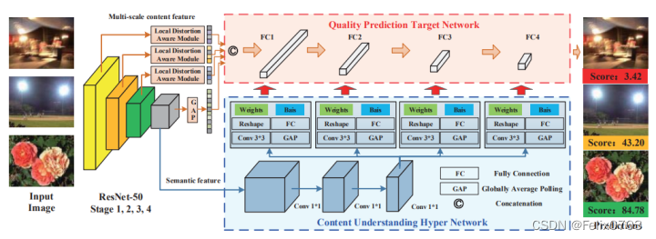
从图中我们可以看到由三个部分组成:
(1)、resnet50进行第一步的特征提取,提取语义信息。
(2)、获取到的特征进行hypernet超网络自适应地建立感知规则
(3)、从hypernet网络中学习到的权重与偏置提供到质量预测网络进行图像质量预测。
接下来知道了整个模糊度判断的网络构成后,我们在代码中进行详细解读。
一、resnet50提取语义信息:
下面进行网络解读,这里有小伙伴可能上一章节训练出了问题,这里面可以看到进行了通道的修改后训练就可以完成了。
class ResNetBackbone(nn.Module):

    def __init__(self, lda_out_channels, in_chn, block, layers, num_classes=1000):
        super(ResNetBackbone, self).__init__()
        self.inplanes = 64
        self.conv1 = nn.Conv2d(3, 64, kernel_size=7, stride=2, padding=3, bias=False)
        self.bn1 = nn.BatchNorm2d(64)
        self.relu = nn.ReLU(inplace=True)
        self.maxpool = nn.MaxPool2d(kernel_size=3, stride=2, padding=1)
        self.layer1 = self._make_layer(block, 64, layers[0])
        self.layer2 = self._make_layer(block, 128, layers[1], stride=2)
        self.layer3 = self._make_layer(block, 256, layers[2], stride=2)
        self.layer4 = self._make_layer(block, 512, layers[3], stride=2)

        #局部失真感知模块
        self.lda1_pool = nn.Sequential(
            nn.Conv2d(256, 16, kernel_size=1, stride=1, padding=0, bias=False),
            nn.AvgPool2d(7, stride=7),
        )
        #这里原来网络是适配的224*224的尺寸,现在我们要改为384*128尺寸,因此需要改一下输入的通道
        self.lda1_fc = nn.Linear(832, lda_out_channels)#224*224尺寸  16 * 64

        self.lda2_pool = nn.Sequential(
            nn.Conv2d(512, 32, kernel_size=1, stride=1, padding=0, bias=False),
            nn.AvgPool2d(7, stride=7),
        )
        self.lda2_fc = nn.Linear(384, lda_out_channels)#224*224尺寸  32 * 16

        self.lda3_pool = nn.Sequential(
            nn.Conv2d(1024, 64, kernel_size=1, stride=1, padding=0, bias=False),
            nn.AvgPool2d(7, stride=7),
        )
        self.lda3_fc = nn.Linear(192, lda_out_channels)#224*224尺寸  64 * 4

        self.lda4_pool = nn.AvgPool2d(3, stride=3)#224*224尺寸 7,stride=7
        self.lda4_fc = nn.Linear(8192, in_chn - lda_out_channels * 3)#224*224 2048

        for m in self.modules():
            if isinstance(m, nn.Conv2d):
                n = m.kernel_size[0] * m.kernel_size[1] * m.out_channels
                m.weight.data.normal_(0, math.sqrt(2. / n))
            elif isinstance(m, nn.BatchNorm2d):
                m.weight.data.fill_(1)
                m.bias.data.zero_()

        #参数初始化
        nn.init.kaiming_normal_(self.lda1_pool._modules['0'].weight.data)
        nn.init.kaiming_normal_(self.lda2_pool._modules['0'].weight.data)
        nn.init.kaiming_normal_(self.lda3_pool._modules['0'].weight.data)
        nn.init.kaiming_normal_(self.lda1_fc.weight.data)
        nn.init.kaiming_normal_(self.lda2_fc.weight.data)
        nn.init.kaiming_normal_(self.lda3_fc.weight.data)
        nn.init.kaiming_normal_(self.lda4_fc.weight.data)

    def _make_layer(self, block, planes, blocks, stride=1):
        downsample = None
        if stride != 1 or self.inplanes != planes * block.expansion:
            downsample = nn.Sequential(
                nn.Conv2d(self.inplanes, planes * block.expansion,
                          kernel_size=1, stride=stride, bias=False),
                nn.BatchNorm2d(planes * block.expansion),
            )

        layers = []
        layers.append(block(self.inplanes, planes, stride, downsample))
        self.inplanes = planes * block.expansion
        for i in range(1, blocks):
            layers.append(block(self.inplanes, planes))

        return nn.Sequential(*layers)

    def forward(self, x):
        x = self.conv1(x)
        x = self.bn1(x)
        x = self.relu(x)
        x = self.maxpool(x)
        x = self.layer1(x)

        # 与论文中的lda操作效果相同,但节省更多内存。
        lda_1 = self.lda1_fc(self.lda1_pool(x).view(x.size(0), -1))
        x = self.layer2(x)
        lda_2 = self.lda2_fc(self.lda2_pool(x).view(x.size(0), -1))
        x = self.layer3(x)
        lda_3 = self.lda3_fc(self.lda3_pool(x).view(x.size(0), -1))
        x = self.layer4(x)
        lda_4 = self.lda4_fc(self.lda4_pool(x).view(x.size(0), -1))
        # vec = torch.cat(lda_1,1)
        vec = torch.cat((lda_1, lda_2, lda_3, lda_4), 1)

	    #resnet50网络提取的语义信息
        out = {}
        out['hyper_in_feat'] = x
        out['target_in_vec'] = vec

        return out
这里我们可以看到out的语义信息,形状为(40,2048,12,4),接下来要进入hypernet网络。

二、hypernet超网络自适应地建立感知规则:
我们前面提取到了语义信息之后,我们需要在hypernet中学习新的权重和偏置,给到下一步的质量预测网络中进行模糊度的判断。
这里我们用到了多尺度的特征融合,更好的对小目标进行判断并且由于特征图分辨率较大,物体 的定位也更精准,这也是hypernet的思想。
class HyperNet(BaseBackbone):

    def __init__(self, lda_out_channels, hyper_in_channels, target_in_size, target_fc1_size, target_fc2_size, target_fc3_size, target_fc4_size, feature_size1,feature_size2):
        super(HyperNet, self).__init__()

        self.hyperInChn = hyper_in_channels
        self.target_in_size = target_in_size
        self.f1 = target_fc1_size
        self.f2 = target_fc2_size
        self.f3 = target_fc3_size
        self.f4 = target_fc4_size
        self.feature_size1 = feature_size1
        self.feature_size2 = feature_size2

        self.res = resnet50_backbone(lda_out_channels, target_in_size, pretrained=True)

        self.pool = nn.AdaptiveAvgPool2d((1, 1))

        # resnet 输出特征的卷积层
        self.conv1 = nn.Sequential(
            nn.Conv2d(2048, 1024, 1, padding=(0, 0)),
            nn.ReLU(inplace=True),
            nn.Conv2d(1024, 512, 1, padding=(0, 0)),
            nn.ReLU(inplace=True),
            nn.Conv2d(512, self.hyperInChn, 1, padding=(0, 0)),
            nn.ReLU(inplace=True)
        )

        # hypernet超网络部分,conv 用于生成目标 fc 的权重,fc 用于生成目标 fc 的偏置
        #这里我们可以看到之前配置文件设定的多种尺度特征大小(192、96、48、24、12、4)
        self.fc1w_conv = nn.Conv2d(self.hyperInChn, int(self.target_in_size * self.f1 / feature_size1 *feature_size2/16), 3,  padding=(1, 1))#** 2
        self.fc1b_fc = nn.Linear(self.hyperInChn, self.f1)
        self.fc2w_conv = nn.Conv2d(self.hyperInChn, int(self.f1 * self.f2 / feature_size1 *feature_size2/16), 3, padding=(1, 1))
        self.fc2b_fc = nn.Linear(self.hyperInChn, self.f2)
        self.fc3w_conv = nn.Conv2d(self.hyperInChn, int(self.f2 * self.f3 / feature_size1 *feature_size2/16), 3, padding=(1, 1))
        self.fc3b_fc = nn.Linear(self.hyperInChn, self.f3)
        self.fc4w_conv = nn.Conv2d(self.hyperInChn, int(self.f3 * self.f4 / feature_size1 *feature_size2/16), 3, padding=(1, 1))
        self.fc4b_fc = nn.Linear(self.hyperInChn, self.f4)

        self.fc5w_conv = nn.Conv2d(self.hyperInChn, int(self.f4**2/ feature_size1 *feature_size2/16), 3, padding=(1, 1))
        self.fc5b_fc = nn.Linear(self.hyperInChn, 1)

        for i, m_name in enumerate(self._modules):
            if i > 2:
                nn.init.kaiming_normal_(self._modules[m_name].weight.data)

    def forward(self, img):
        feature_size1 = self.feature_size1
        feature_size2 = self.feature_size2
        res_out = self.res(img)

        # 目标网络的输入向量
        target_in_vec = res_out['target_in_vec'].view(-1, self.target_in_size, 1, 1)

        # 超网络的输入特征
        hyper_in_feat = self.conv1(res_out['hyper_in_feat']).view(-1, self.hyperInChn, feature_size1, feature_size2)

        # 生成目标权重和偏置
        target_fc1w = self.fc1w_conv(hyper_in_feat).view(-1, self.f1, self.target_in_size, 1, 1)
        target_fc1b = self.fc1b_fc(self.pool(hyper_in_feat).squeeze()).view(-1, self.f1)

        target_fc2w = self.fc2w_conv(hyper_in_feat).view(-1, self.f2, self.f1, 1, 1)
        target_fc2b = self.fc2b_fc(self.pool(hyper_in_feat).squeeze()).view(-1, self.f2)
        #
        target_fc3w = self.fc3w_conv(hyper_in_feat).view(-1, self.f3, self.f2, 1, 1)
        target_fc3b = self.fc3b_fc(self.pool(hyper_in_feat).squeeze()).view(-1, self.f3)

        #
        target_fc4w = self.fc4w_conv(hyper_in_feat).view(-1, self.f4, self.f3, 1, 1)
        target_fc4b = self.fc4b_fc(self.pool(hyper_in_feat).squeeze()).view(-1, self.f4)

        target_fc5w = self.fc5w_conv(hyper_in_feat).view(-1, self.f4, self.f4, 1, 1)
        target_fc5b = self.fc5b_fc(self.pool(hyper_in_feat).squeeze()).view(-1, 1)

        out = {}
        out['target_in_vec'] = target_in_vec
        out['target_fc1w'] = target_fc1w
        out['target_fc1b'] = target_fc1b
        out['target_fc2w'] = target_fc2w
        out['target_fc2b'] = target_fc2b
        out['target_fc3w'] = target_fc3w
        out['target_fc3b'] = target_fc3b
        out['target_fc4w'] = target_fc4w
        out['target_fc4b'] = target_fc4b
        out['target_fc5w'] = target_fc5w
        out['target_fc5b'] = target_fc5b
现在经过hypernet网络后,学习到了权重与偏置接下来就要送到我们的质量预测网络全连接层了,这也是最后一步。

三、质量预测:
现在我们学习到图片的特征权重和偏置之后,到了我们质量预测的阶段了。代码如下:
l1 = nn.Sequential(
            TargetFC(out['target_fc1w'], out['target_fc1b']),
            nn.Sigmoid(),
        )
        l2 = nn.Sequential(
            TargetFC(out['target_fc2w'], out['target_fc2b']),
            nn.Sigmoid(),
        )
        #
        l3 = nn.Sequential(
            TargetFC(out['target_fc3w'], out['target_fc3b']),
            nn.Sigmoid(),
        )
        #
        l4 = nn.Sequential(
            TargetFC(out['target_fc4w'], out['target_fc4b']),
            nn.Sigmoid(),
            TargetFC(out['target_fc5w'], out['target_fc5b']),
            # nn.Linear(24,1)
        )

        q = l1(out['target_in_vec'])
        q = l2(q)
        q = l3(q)
        q = l4(q)#.squeeze()
        return q


class TargetFC(nn.Module):
    """
    目标网络的全连接操作,质量预测。
     注意:
         批次中不同图像的权重和偏差不同,
         因此,在这里我们使用组卷积来批量计算具有单独权重和偏差的图像。
    """
    def __init__(self, weight, bias):
        super(TargetFC, self).__init__()
        self.weight = weight
        self.bias = bias

    def forward(self, input_):

        input_re = input_.view(-1, input_.shape[0] * input_.shape[1], input_.shape[2], input_.shape[3])#224*224尺寸 input_.shape[0] * input_.shape[1]
        weight_re = self.weight.view(self.weight.shape[0] * self.weight.shape[1], self.weight.shape[2], self.weight.shape[3], self.weight.shape[4])
        bias_re = self.bias.view(self.bias.shape[0] * self.bias.shape[1])
        out = F.conv2d(input=input_re, weight=weight_re, bias=None, groups=self.weight.shape[0])
        out1 = out.view(input_.shape[0], self.weight.shape[1], input_.shape[2], input_.shape[3])
        return out1
我们从设定不同的特征尺寸大小进行多尺度的特征融合,使得预测小目标能力更加出色,并且由于特征图分辨率较大,物体的定位也更精准。


 3517
3517


 被折叠的 条评论
为什么被折叠?
被折叠的 条评论
为什么被折叠?
 到【灌水乐园】发言


