深度学习识别手势

Assignment 3

Sign Language Image Classification using Deep Learning

Scenario

A client is interested in having you (or rather the company that you work for) investigate whether it is possible to develop an app that would enable American sign language to be translated for people that do not sign, or those that sign in different languages/styles. They have provided you with a labelled data of images related to signs (hand positions) that represent individual letters in order to do a preliminary test of feasibility.

Your manager has asked you to do this feasibility assessment, but subject to a constraint on the computational facilities available. More specifically, you are asked to do no more than 100 training runs in total (including all models and hyperparameter settings that you consider).

The task requires you to create a Jupyter Notebook to perform 22 steps. These steps involve loading the dataset, fixing data problems, converting labels to one-hot encoding, plotting sample images, creating, training, and evaluating two sequential models with 20 Dense layers with 100 neurons each, checking for better accuracy using MC Dropout, retraining the first model with performance scheduling, evaluating both models, using transfer learning to create a new model using pre-trained weights, freezing the weights of the pre-trained layers, adding new Dense layers, training and evaluating the new model, predicting and converting sign language to text using the best model.

IMPORTANT

• Train all the models locally on your own machine. No model training should occur on Gradescope (GS).
• After completing the training, upload the trained models' h5 files and their training histories along with your notebook to GS.
  • best_dnn_bn_model.h5
  • best_dnn_bn_perf_model.h5
  • best_dnn_selu_model.h5
  • best_mobilenet_model.h5
  • history1
  • history2
  • history1_perf
  • historymb
• To avoid any confusion and poor training on GS, please remember to comment out the training code in your notebook before uploading it to GS.

In [1]:

# import the necessary libraries (TensorFlow, sklearn NumPy, Pandas, and Matplotlib)

import tensorflow as tf
from tensorflow import keras
import numpy as np
import pandas as pd
import matplotlib.pyplot as plt
import os

# Install opencv using "pip install opencv-python" in order to use cv2.
import cv2

Step0 This test is for checking whether all the required files are submitted. Once you submit all the required files to the autograder, you will be able to pass this step.

IMPORTANT: Run this step to determine whether you have created all the required files correctly.

Points: 1

In [2]:

# Don't change this cell code
required_files = ['best_dnn_bn_model.h5','best_dnn_bn_perf_model.h5','best_dnn_selu_model.h5','best_mobilenet_model.h5','history1','history2','history1_perf','historymb']
step0_files = True
for file in required_files:
    if os.path.exists(file) == False:
        step0_files = False
        print("One or more files are missing!")
        break

# The following code is used by the autograder. Do not modify it.   
step0_data = step0_files

grader.check("step00")

Data Preprocessing

STEP1 Load the dataset (train and test) using Pandas from the CSV file.

Points: 1

In [3]:

# Load the dataset using Pandas from the CSV file
train_df = pd.read_csv("sign_mnist_train.csv")
test_df = pd.read_csv("sign_mnist_test.csv")

# The following code is used by the autograder. Do not modify it.
step1_sol = test_df.shape

train_df.head()

Out[3]:

	label	pixel1	pixel2	pixel3	pixel4	pixel5	pixel6	pixel7	pixel8	pixel9	...	pixel775	pixel776	pixel777	pixel778	pixel779	pixel780	pixel781	pixel782	pixel783	pixel784
0	3	107	118	127	134	139	143	146	150	153	...	207	207	207	207	206	206	206	204	203	202
1	6	155	157	156	156	156	157	156	158	158	...	69	149	128	87	94	163	175	103	135	149
2	2	187	188	188	187	187	186	187	188	187	...	202	201	200	199	198	199	198	195	194	195
3	2	211	211	212	212	211	210	211	210	210	...	235	234	233	231	230	226	225	222	229	163
4	13	164	167	170	172	176	179	180	184	185	...	92	105	105	108	133	163	157	163	164	179

5 rows × 785 columns

grader.check("step01")

STEP2 Examine the data and fix any problems. It is important that you don't have gaps in the number of classes, therefore, check the classes which are not available and shift the labels in order to ensure 24 classes, starting from class 0. In addition, normalize the values of your images in a range of 0 and 1.

Points: 1

In [4]:

# Separate labels and pixel values in training and testing sets
train_df = train_df[train_df.label <= 24]

train_labels = train_df.iloc[:, 0].apply(lambda x: x-1 if x > 9 else x).values
test_labels = test_df.iloc[:, 0].apply(lambda x: x-1 if x > 9 else x).values
train_images = (train_df.iloc[:, 1:] / 255.0).values
test_images = (test_df.iloc[:, 1:] / 255.0).values

# The following code is used by the autograder. Do not modify it.
step2_sol = (np.max(train_images)-np.min(train_images), np.max(train_labels)-np.min(train_labels), np.max(test_images)-np.min(test_images), np.max(test_labels)-np.min(test_labels))
step2_sol
# train_labels.value_counts().sort_index()
# # train_images.head()
# type(train_labels), train_images.dtypes, step2_sol
# type(train_labels)

Out[4]:

(1.0, 23, 1.0, 23)

grader.check("step02")

STEP3 Convert Labels to One-Hot Encoding both train and test.

Points: 1

In [5]:

# Convert labels to one-hot encoding
train_labels_encoded = keras.utils.to_categorical(train_labels)
test_labels_encoded = keras.utils.to_categorical(test_labels)

# The following code is used by the autograder. Do not modify it.
step3_sol = (len(np.unique(train_labels_encoded)), len(np.unique(test_labels_encoded)))

test_labels_encoded[:5]

Out[5]:

array([[0., 0., 0., 0., 0., 0., 1., 0., 0., 0., 0., 0., 0., 0., 0., 0.,
        0., 0., 0., 0., 0., 0., 0., 0.],
       [0., 0., 0., 0., 0., 1., 0., 0., 0., 0., 0., 0., 0., 0., 0., 0.,
        0., 0., 0., 0., 0., 0., 0., 0.],
       [0., 0., 0., 0., 0., 0., 0., 0., 0., 1., 0., 0., 0., 0., 0., 0.,
        0., 0., 0., 0., 0., 0., 0., 0.],
       [1., 0., 0., 0., 0., 0., 0., 0., 0., 0., 0., 0., 0., 0., 0., 0.,
        0., 0., 0., 0., 0., 0., 0., 0.],
       [0., 0., 0., 1., 0., 0., 0., 0., 0., 0., 0., 0., 0., 0., 0., 0.,
        0., 0., 0., 0., 0., 0., 0., 0.]], dtype=float32)

grader.check("step03")

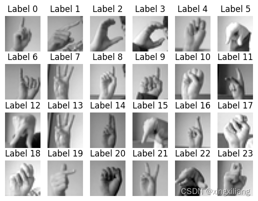
STEP4 Plot one sample image for each letter in the dataset given in the training set. To solve this step you should use the function imshow to diplay your images in a similar to the image below.

Points: 0

In [6]:

# Get one sample image for each label
images = []
index = 0;
for i in range(0, 25):
#     print(i)
    if i != 9:
        one_pic = train_df[train_df.label == i].iloc[0, 1:]
#         print(one_pic.shape, type(one_pic))
        images.append(one_pic.values.reshape(28, 28))
        
        row = index // 6
        col = index % 6
        plt.subplot2grid((4, 6), (row, col))
        plt.imshow(images[-1], cmap=plt.get_cmap('gray'))
        plt.axis("off")
        plt.title(f"Label {index}")
        index += 1

    
plt.show()
# Plot the sample images
train_df.head()

Out[6]:

	label	pixel1	pixel2	pixel3	pixel4	pixel5	pixel6	pixel7	pixel8	pixel9	...	pixel775	pixel776	pixel777	pixel778	pixel779	pixel780	pixel781	pixel782	pixel783	pixel784
0	3	107	118	127	134	139	143	146	150	153	...	207	207	207	207	206	206	206	204	203	202
1	6	155	157	156	156	156	157	156	158	158	...	69	149	128	87	94	163	175	103	135	149
2	2	187	188	188	187	187	186	187	188	187	...	202	201	200	199	198	199	198	195	194	195
3	2	211	211	212	212	211	210	211	210	210	...	235	234	233	231	230	226	225	222	229	163
4	13	164	167	170	172	176	179	180	184	185	...	92	105	105	108	133	163	157	163	164	179

5 rows × 785 columns

grader.check("step04")

Create Neural Network Architectures

In this part you should create two different models (model1 and model2) with different architectures.

STEP5 Create one sequential model in TensorFlow with 20 Dense layers with 100 neurons each one. Consider the specific modifications that you need to do in order to work with your specific input and those to get the required output.

• This model uses Batch Normalization in each layer and uses He initialization. Add Swish activation function to each layer.

Points: 5

In [7]:

import tensorflow as tf
from tensorflow.keras.layers import Dense, BatchNormalization
from tensorflow.keras.activations import swish
from tensorflow.keras.layers import InputLayer, AlphaDropout

# Model 1: with Batch Normalization

layers = []

for i in range(20):
    layers.append(keras.layers.Dense(100, kernel_initializer = 'he_normal'))
    layers.append(keras.layers.Activation("swish"))
    layers.append(keras.layers.BatchNormalization())
layers.append(keras.layers.Dense(24, activation=keras.activations.softmax))
    
model1 = keras.models.Sequential(layers)

# The following code is used by the autograder. Do not modify it.
step5_sol = model1

# for layer in step5_sol.layers:
#     print(isinstance(layer, keras.layers.Activation) , 
#           type(layer))
# #           layer.activation.__name__)
                  

print(any(isinstance(layer, keras.layers.Activation) 
                  and layer.activation.__name__ == 'swish' 
                  for layer in step5_sol.layers))

type(step5_sol)

True

Out[7]:

keras.engine.sequential.Sequential

grader.check("step05")

STEP6 Create a second sequential model in TensorFlow also with 20 Dense layers with 100 neurons each one. Consider the specific modifications that you need to do in order to work with your specific input and those to get the required output.

In this model you should:

• Replace Batch Normalization with SELU and make necessary adjustments to ensure the network self-normalizes, use LeCun normal initialization, make sure the DNN contains only a sequence of dense layers.
• Regularize this model with Alpha Dropout 0.1.

Points: 5

In [8]:

# Model 2: with SELU and self-normalization
layers = []

for i in range(20):
    layers.append(keras.layers.Dense(100, activation=keras.activations.selu, 
                                     kernel_initializer = keras.initializers.lecun_normal))
    if i >= 18 or i == 0:
        layers.append(keras.layers.AlphaDropout(rate=0.1))

layers.append(keras.layers.Dense(24, activation=keras.activations.softmax))
# model1.compile(loss=keras.losses.categorical_crossentropy, optimizer='nadam', metrics=['accuracy'])
    
model2 = keras.models.Sequential(layers)

# The following code is used by the autograder. Do not modify it.
step6_sol = model2

namesss = [step6_sol.get_config()['layers'][x]['class_name'] for x in range(1,10)]
print(any('AlphaDropout' in layer for layer in namesss))

# for layer in step5_sol.layers:
#     print(isinstance(layer, keras.layers.Activation) , 
#           type(layer))
#           layer.activation.__name__)
# namesss

True

grader.check("step06")

Compile the Models

STEP7 Compile the both previous models using Nadam optimization. Also:

• Set the loss function to categorical cross-entropy.
• Set the metric to accuracy.

Points: 2

In [9]:

# Compile first model
model1.compile(loss='categorical_crossentropy', optimizer='nadam', metrics=['accuracy'])

# history = model1.fit(train_images, train_labels_encoded)
# Compile second model
model2.compile(loss='categorical_crossentropy', optimizer='nadam', metrics=['accuracy'])

# The following code is used by the autograder. Do not modify it.
step7_sol = (model1.loss,model2.loss,model1.optimizer.get_config()['name'],model2.optimizer.get_config()['name'])

step7_sol[0]

('categorical_crossentropy' in step7_sol[0])

Out[9]:

True

grader.check("step07")

Model Training

STEP8 One of these models work preferably with data, which follow a normal distribution. Generate train_images_scaled and test_images_scaled using a Sklearn function that allow you to convert data to a normal distribution with mean 0 and variance equal 1.

Points: 2

In [10]:

from sklearn.preprocessing import StandardScaler


scaler = StandardScaler()
if train_images.dtype != np.dtype('int32'):
    train_images = train_images * 255.0
    train_images = train_images.astype(int)
    test_images = test_images * 255.0
    test_images = test_images.astype(int)

train_images_scaled = scaler.fit_transform(train_images)
test_images_scaled = scaler.transform(test_images)

# The following code is used by the autograder. Do not modify it.
step8_sol = (np.mean(train_images_scaled),np.mean(test_images_scaled),np.std(train_images_scaled),np.std(test_images_scaled))


train_images[:3]

Out[10]:

array([[107, 118, 127, ..., 204, 203, 202],
       [155, 157, 156, ..., 103, 135, 149],
       [187, 188, 188, ..., 195, 194, 195]])

grader.check("step08")

STEP9 Train the two models on the training dataset using early stopping. In order to save the results given by your training for your models, create checkpoints saving the best model in each case using the function ModelCheckpoint. Note that one of the models use the scaled data obtained in STEP8. Meanwhile, the other model does not. Figure out which is the proper input data for each model.

• Limit the number of epochs to 100. Set the batch size to or greater than 32.

IMPORTANT: Comment out the code to train/fit the two models. Keep the code given to save the models.

Points: 3

In [11]:

import pickle

# The following line of code is used by the autograder. Do not modify it.
history1, history2 = None, None
 
# We go to set a seed to get the same results every run
np.random.seed(42)
tf.random.set_seed(42)

# split 
from sklearn.model_selection import train_test_split

# Split the data
train_images_scaled_pure, val_images_scaled, train_labels_pure, val_labels = train_test_split(train_images_scaled, 
                                                                                    train_labels_encoded, 
                                                                                    test_size=0.2, 
                                                                                    random_state=42)
train_images_pure_0, val_images_0, train_labels_pure_0, val_lables_0 = train_test_split(train_images,train_labels_encoded,
                                                                     test_size = 0.2, 
                                                                     random_state = 42)


# Set up early stopping
early_stopping = keras.callbacks.EarlyStopping(patience=10,
                                                  restore_best_weights=True)

# Define model checkpoint callback
model1_checkpoint_cb = keras.callbacks.ModelCheckpoint("best_dnn_bn_model.h5",
                                                save_best_only=True)
model2_checkpoint_cb = keras.callbacks.ModelCheckpoint("best_dnn_selu_model.h5",
                                                save_best_only=True)

#################################### Perform the training on your machine and then comment out the following section before uploading it to gradescope. 
# Make sure your best model is named as follows:
# Model1 filename = best_dnn_bn_model.h5
# Model2 filename = best_dnn_selu_model.h5

# # Train model 1 (Comment this out before submission)
# history1 = model1.fit(train_images_pure_0, train_labels_pure_0,
#                         epochs=100,
#                         validation_data=(val_images_0, val_lables_0),
#                         callbacks=[model1_checkpoint_cb, early_stopping])

# Train model 2 (Comment this out before submission)
# history2 =  model2.fit(train_images_scaled_pure, train_labels_pure,
#                         epochs=100,
#                         validation_data=(val_images_scaled, val_labels),
#                         callbacks=[model2_checkpoint_cb, early_stopping])

# # The following code will save your history - don't change it.
# if 'history1' in globals():  
#     with open('./history1', 'wb') as file_pi:
#         pickle.dump(history1.history, file_pi)
# if 'history2' in globals():  
#     with open('./history2', 'wb') as file_pi:
#         pickle.dump(history2.history, file_pi)
####################################

# The following code is used by the autograder. Do not modify it.
step9_sol = (model1_checkpoint_cb, model2_checkpoint_cb, early_stopping)

train_images_pure_0[:4]

Out[11]:

array([[152, 153, 156, ..., 196, 193, 192],
       [ 60,  62,  68, ..., 156, 155, 153],
       [ 76,  84,  94, ..., 105,  88,  88],
       [169, 171, 172, ...,  85,  58,  42]])

grader.check("step09")

STEP10 Using the loaded models obtained from the code given below, evaluate the performance of each model on the test set. While evaluating, make sure to take into account which model uses scaled data and which model does not.

Points: 2

In [12]:

# Do not change the following 4 lines of code.
# define the file name for the saved model
model1_name = "best_dnn_bn_model.h5"
# load the model
model1 = keras.models.load_model(model1_name)
# define the file name for the saved model
model2_name = "best_dnn_selu_model.h5"
# load the model
model2 = keras.models.load_model(model2_name)

# Evaluate the models on the test set
test_loss1, test_acc1 = model1.evaluate(test_images, test_labels_encoded)
test_loss2, test_acc2 = model2.evaluate(test_images_scaled, test_labels_encoded)
print(f"Model 1| Test accuracy: {test_acc1:.4f}, Test loss: {test_loss1:.4f}")
print(f"Model 2| Test accuracy: {test_acc2:.4f}, Test loss: {test_loss2:.4f}")

# The following code is used by the autograder. Do not modify it.
step10_sol = (test_loss1, test_acc1, test_loss2, test_acc2, model1, model2)

225/225 [==============================] - 1s 2ms/step - loss: 1.7584 - accuracy: 0.6673
225/225 [==============================] - 0s 1ms/step - loss: 1.2951 - accuracy: 0.8233
Model 1| Test accuracy: 0.6673, Test loss: 1.7584
Model 2| Test accuracy: 0.8233, Test loss: 1.2951

grader.check("step10")

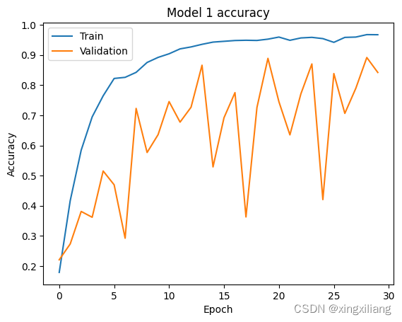
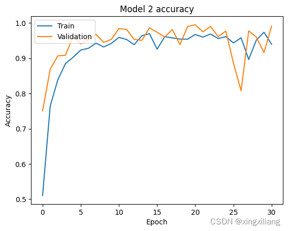
STEP11 From the loaded history of the two trained models, plot a graph of accuracy vs number of epochs for both training and validation.

Points: 0

In [13]:

# Load history for model 1 (Do not modify this code)
history_name1 = "./history1"
with open(history_name1, "rb") as file_pi:
    loaded_history1 = pickle.load(file_pi)
    
# Load history for model 2 (Do not modify this code)
history_name2 = "./history2"
with open(history_name2, "rb") as file_pi:
    loaded_history2 = pickle.load(file_pi)

# Plot the training and validation accuracies during training for both models
plt.plot(loaded_history1['accuracy'])
plt.plot(loaded_history1['val_accuracy'])
plt.title('Model 1 accuracy')
plt.ylabel('Accuracy')
plt.xlabel('Epoch')
plt.legend(['Train', 'Validation'], loc='upper left')
plt.show()

plt.plot(loaded_history2['accuracy'])
plt.plot(loaded_history2['val_accuracy'])
plt.title('Model 2 accuracy')
plt.ylabel('Accuracy')
plt.xlabel('Epoch')
plt.legend(['Train', 'Validation'], loc='upper left')


# The following code is used by the autograder. Do not modify it.
step11_sol = (loaded_history1, loaded_history2)

grader.check("step11")

MC Dropout

STEP12 Check if model2 achieves better accuracy using MC Dropout (without retraining).

Points: 3

In [14]:

#This function computes the MC (Monte Carlo) Dropout predictions for a given model and input data. 
# It returns the mean of multiple predictions obtained by running the model in training mode.
#Parameters
#   model: A trained model with a dropout layers.
#   X    : The input data for which the predictions are to be made.
#   n_samples: The number of Monte Carlo samples to generate..
#Returns
  # The function returns an array-like object containing the MC Dropout predictions for the given input data. 
  # The shape of the output should be the same as the model's output layer.
def mc_dropout_predict(model, X, n_samples=20):
    # Write your code here
    y_probas = np.stack([model(X, training=True)
                     for sample in range(n_samples)])
    output_mc = y_probas.mean(axis=0) 
    return output_mc

# model2.evaluate(test_images_scaled, test_labels_encoded)
# call mc_dropout_predict to Compute the MC Dropout predictions for model 2
output_mc = mc_dropout_predict(model2, test_images_scaled, 90)

# Compute the accuracy using MC Dropout
accuracy_mc = np.mean(test_labels == output_mc.argmax(axis=1))

# Display result.
print(f"Model 2 with MC Dropout: Test accuracy: {accuracy_mc:.4f}")

# The following code is used by the autograder. Do not modify it.
step12_sol = (output_mc, accuracy_mc)

test_labels_encoded.argmax(axis=1).shape

Model 2 with MC Dropout: Test accuracy: 0.8260

Out[14]:

(7172,)

grader.check("step12")

Learning Rate (LR) scheduling

STEP13 Retrain model1 using performance scheduling and see if it improves training speed and model accuracy.

IMPORTANT: Define the model the same way model1 was defined and compile the model the same way as model1.

Points: 2

In [15]:

from tensorflow.keras.callbacks import ReduceLROnPlateau

# Do not modify the following line of code.
history1_perf = None

# Redefine Model 1 so we start again with random weights
layers = []

for i in range(20):
    layers.append(keras.layers.Dense(100, activation=keras.activations.swish, kernel_initializer = 'he_normal'))
    layers.append(keras.layers.BatchNormalization())
layers.append(keras.layers.Dense(24, activation=keras.activations.softmax))

model1_perfLRS = keras.models.Sequential(layers)

# Compile the model with Nadam optimizer and categorical cross-entropy loss
model1_perfLRS.compile(loss=keras.losses.categorical_crossentropy, optimizer="nadam", metrics=['accuracy'])

# Define the learning rate schedule
lr_scheduler = keras.callbacks.ReduceLROnPlateau(factor=0.5, patience=5) 

# Creating model checkpoint to save the best model. 
dnn_bn_perf_checkpoint_cb =  keras.callbacks.ModelCheckpoint("best_dnn_bn_perf_model.h5",
                                                save_best_only=True)

#####Perform the training on your machine and then comment out the following section before uploading it to gradescope.
####################################  
# Make sure your best model is named as follows:
# Model1 with performance scheduling filename = best_dnn_bn_perf_model.h5


# Train the model using early stopping and exponential scheduling (Comment this out before submission)
# history1_perf = model1_perfLRS.fit(train_images_pure_0, train_labels_pure_0,
#                                    epochs=100,
#                                    validation_data=(val_images_0, val_lables_0), 
#                                    callbacks=[dnn_bn_perf_checkpoint_cb, early_stopping, lr_scheduler])
# #                             callbacks=[dnn_bn_perf_checkpoint_cb, early_stopping， lr_scheduler])

# # The following code will save your history - don't change it - comment it out before uploading to GS
# if "history1_perf" in globals():
#     with open('./history1_perf', 'wb') as file_pi:
#         pickle.dump(history1_perf.history, file_pi)
####################################
# The following code is used by the autograder. Do not modify it.
step13_sol = (dnn_bn_perf_checkpoint_cb, lr_scheduler)

grader.check("step13")

STEP14 Using the loaded model obtained from the code given below, evaluate the performance of the model on the test set.

Points: 1

In [16]:

# Do not change the following 2 lines of code.
# define the file name for the saved model
model_name = "best_dnn_bn_perf_model.h5"
# load the model
model1_perf = keras.models.load_model(model_name)

# Evaluate the model on the test set
test_loss1_perf, test_acc1_perf = model1_perf.evaluate(test_images, test_labels_encoded)
print(f"Model 1 with performance scheduling: Test accuracy: {test_acc1_perf:.4f}")

# The following code is used by the autograder. Do not modify it.
step14_sol = (test_loss1_perf, test_acc1_perf)

225/225 [==============================] - 1s 2ms/step - loss: 0.9349 - accuracy: 0.8134
Model 1 with performance scheduling: Test accuracy: 0.8134

grader.check("step14")

STEP15 From the history of the models loaded using the code given below, plot a graph of accuracy vs number of epochs for both training and validation.

Points: 0

In [17]:

# load history for model 1 with learning rate scheduling (do not modify the following code)
history_name1_perf = "./history1_perf"
with open(history_name1_perf, "rb") as file_pi:
    loaded_history1_perf = pickle.load(file_pi)

# Load history for the original model1 (do not modify the following code)
history_name1 = "./history1"
with open(history_name1, "rb") as file_pi:
    loaded_history1 = pickle.load(file_pi)

# Plot the training and validation accuracy for both models
plt.plot(loaded_history1_perf['accuracy'])
plt.plot(loaded_history1_perf['val_accuracy'])
plt.title('Model with LR perf accuracy')
plt.ylabel('Accuracy')
plt.xlabel('Epoch')
plt.legend(['Train', 'Validation'], loc='upper left')
plt.show()

plt.plot(loaded_history1['accuracy'])
plt.plot(loaded_history1['val_accuracy'])
plt.title('Model 1 accuracy')
plt.ylabel('Accuracy')
plt.xlabel('Epoch')
plt.legend(['Train', 'Validation'], loc='upper left')

Out[17]:

<matplotlib.legend.Legend at 0x210936d6190>

grader.check("step15")

Transfer learning

Use transfer learning by using a pre-trained MobileNetV3Small model on imagenet dataset, and fine-tuning it on the Sign Language MNIST dataset.

STEP16 First of all, you to prepare your data for this model.

• Reshape your input data (train and test) to (28, 28, 3).
• Standardize your input.

Points: 2

In [18]:

# Reshape train data to (num_samples, 28, 28, 3)
n = len(train_images)
train_images_mb = train_images.reshape(n, 28, 28)
train_images_mb = np.stack([train_images_mb, train_images_mb, train_images_mb], axis=3)

# Reshape test data to (num_samples, 28, 28, 3)
n = len(test_images)
test_images_mb = test_images.reshape(n, 28, 28)
test_images_mb = np.stack([test_images_mb, test_images_mb, test_images_mb], axis=3)

# The following code is used by the autograder. Do not modify it.
step16_sol = (train_images_mb,test_images_mb)
test_images_mb.shape
# Get one sample image for each label
images = []
index = 0;
for i in range(0, 24):
#     print(i)
    if True:
        one_pic = train_images_mb[i, :, :, :]
#         print(one_pic.shape, type(one_pic))
        images.append(one_pic)
        
        row = index // 6
        col = index % 6
        plt.subplot2grid((4, 6), (row, col))
        plt.imshow(images[-1])
        plt.axis("off")
        plt.title(f"Label {index}")
        index += 1

    
plt.show()

test_images[:3]

Out[18]:

array([[149, 149, 150, ..., 112, 120, 107],
       [126, 128, 131, ..., 184, 182, 180],
       [ 85,  88,  92, ..., 225, 224, 222]])

grader.check("step16")

Step17 Now, we need to define and set up the model. For this you need to follow the next steps:

• Load the pre-trained MobileNetV3Small model with weights from ImageNet.
• Freeze the weights of the pretrained layers.
• Modify the input layer to accept inputs of shape (28, 28, 3).
• Also, add layer UpSampling2D to upscale the input by a factor of 2.

Consider that maybe you need to adapt the default output.

Points: 2

In [25]:

from tensorflow.keras.applications import MobileNetV3Small 
from tensorflow.keras.layers import GlobalAveragePooling2D, Dense

# Load the pre-trained MobileNet model with weights from ImageNet
base_mb_model =  MobileNetV3Small(weights='imagenet', include_top=False, input_shape=(56, 56, 3))

# Freeze the weights of the pre-trained layers
for layer in base_mb_model.layers:
    layer.trainable = False

# Create the new model
final_mb_model = keras.models.Sequential()
final_mb_model.add(keras.layers.UpSampling2D(size=(2, 2), input_shape=(28, 28, 3)))
final_mb_model.add(base_mb_model)

# Add a global average pooling layer
final_mb_model.add(GlobalAveragePooling2D())
final_mb_model.add(Dense(128, activation='relu'))
# final_mb_model.add(Dense(128, activation='relu'))
final_mb_model.add(keras.layers.Dense(24, activation=keras.activations.softmax))


# The following code is used by the autograder. Do not modify it.
step17_sol = final_mb_model

WARNING:tensorflow:`input_shape` is undefined or non-square, or `rows` is not 224. Weights for input shape (224, 224) will be loaded as the default.

grader.check("step17")

Step18 Once we define the model and do the specific modifications to adjust to our data, we compile it.

• Use a learning rate schedule that uses an exponential decay schedule.
• Compile and train the model.

Points: 2

In [26]:

from tensorflow.keras.optimizers.schedules import ExponentialDecay
from tensorflow.keras.optimizers import Adam

# Define an initial learning rate                            
initial_learning_rate = 0.01


def exponential_decay(lr0, s):
    def exponential_decay_fn(epoch):
        return lr0 * 0.1**(epoch / s)
    return exponential_decay_fn

# Create the proper learning rate schedule
fn = exponential_decay(lr0 = initial_learning_rate, s = 20)
lr_schedule = keras.callbacks.LearningRateScheduler(fn)


# Define the learning rate schedule
lr_schedule = ExponentialDecay(
    initial_learning_rate=0.01,
    decay_steps=20,
    decay_rate=0.1, # 0.1, 0.9
    staircase=True)

# Define the optimizer with the learning rate schedule
# adam_op = Adam(learning_rate=lr_schedule)


# Compile model
sgd_op = keras.optimizers.SGD(learning_rate=0.01) # the default lr is 1e-2
final_mb_model.compile(loss="categorical_crossentropy", optimizer="Nadam",
                     metrics=["accuracy"]) 

# The following code is used by the autograder. Do not modify it.
step18_sol = (lr_schedule, final_mb_model)

isinstance(step18_sol[0], keras.optimizers.schedules.ExponentialDecay), ('Nadam' in step18_sol[1].optimizer.get_config()['name'])

Out[26]:

(True, True)

grader.check("step18")

Step19 Train the mobilenet model. Include early stopping in your training procedure.

Points: 2

In [28]:

# Do not modify the following line of code.
history_mb = None

# Define model checkpoint callback (Do not modify this code).
best_model_checkpoint = keras.callbacks.ModelCheckpoint("best_mobilenet_model.h5",
                                                save_best_only=True)

# Set up early stopping
early_stopping_cb = keras.callbacks.EarlyStopping(patience=10,
                                                  restore_best_weights=True)


train_images_pure_mb, val_images_mb, train_labels_pure_mb, val_lables_mb = train_test_split(train_images_mb,train_labels_encoded,
                                                                     test_size = 0.2, 
                                                                     random_state = 42)

## Perform the training on your machine and then comment out the following section before uploading it to gradescope. 
#################################### 
# make sure your best model is named as follow:
# MobileNet model filename = best_mobilenet_model.h5
# Train the model (comment this section out)
# history_mb = final_mb_model.fit(train_images_pure_mb, train_labels_pure_mb,
#                                    epochs=50,
#                                    validation_data=(val_images_mb, val_lables_mb), 
#                                    callbacks=[best_model_checkpoint, early_stopping_cb])

# # The following code will save your history - don't change it
# if "history_mb" in globals():
#     with open('./historymb', 'wb') as file_pi:
#         pickle.dump(history_mb.history, file_pi)    
####################################

# The following code is used by the autograder. Do not modify it.
step19_sol = (best_model_checkpoint, early_stopping_cb)

grader.check("step19")

Step20 For the trained model loaded using the code given below, evaluate its performance on the test set.

Points: 1

In [29]:

# Do not modify the following two lines of code.
# define the file name for the saved model
model_name = "best_mobilenet_model.h5"
# load the model
final_mb_model = keras.models.load_model(model_name)

# Reshape the input data to (num_samples, 28, 28, 3)

# Evaluate the model on the test set
test_loss1_mobilenet, test_acc1_mobilenet = final_mb_model.evaluate(test_images_mb, test_labels_encoded)
print(f"Model Mobile Net: Test accuracy: {test_acc1_mobilenet:.4f}")

# The following code is used by the autograder. Do not modify it.
step20_sol = (test_loss1_mobilenet,test_acc1_mobilenet)

225/225 [==============================] - 4s 15ms/step - loss: 0.4878 - accuracy: 0.9067
Model Mobile Net: Test accuracy: 0.9067

grader.check("step20")

Step21 So far, you have seen the overall performance of your models. However, it is possible that some classes may be more difficult to classify than others. To gain a clearer understanding of which letters are the most difficult or easiest to predict, you can use your MobileNet model and make predictions on your test data using the predict function. Based on this, you can check the proportion of correct matches for each letter over the total number of that specific letter in the test data (as the proportion of one letter may differ from that of others). Finally, return the result as a string indicating the most complex and easiest letter to predict based on our analysis (e.g., "a" in lowercase).

Points: 2

In [30]:

from sklearn.metrics import classification_report
import string

# Put here again the labels (not hot encoded)
test_labels = test_labels

# Make the prediction using MobileNet model. Use the function predict.
predictions = final_mb_model.predict(test_images_mb)
prediction_test = np.argmax(predictions, axis=1)

from sklearn.metrics import confusion_matrix

# Calculate confusion matrix
confusion_mtx = confusion_matrix(test_labels, prediction_test) 

# Calculate per-class accuracy from the confusion matrix
per_class_accuracy = confusion_mtx.diagonal() / confusion_mtx.sum(axis=1)

# Create a mapping of class labels to class indices
class_labels = list(string.ascii_lowercase)
class_labels.remove('z')
class_labels.remove('j')

# Create a dictionary of class labels and their corresponding accuracy
class_accuracy = dict(zip(class_labels, per_class_accuracy))
easiest_class = max(class_accuracy, key=class_accuracy.get)
hardest_class = min(class_accuracy, key=class_accuracy.get)

# What is the most difficult letter to predict? (if you have many letters which are equally difficult to predict, pick up any of them. Only one and put in a string (e.g. "a"))
complex_letter = hardest_class

# What is the easist letter to predict? (if you have many letters which are equally easy to predict, pick up any of them. Only one and put in a string (e.g. "a"))
easiest_letter = easiest_class

# The following code is used by the autograder. Do not modify it.
step21_sol = (test_labels,prediction_test,complex_letter,easiest_letter)

class_accuracy, step21_sol

225/225 [==============================] - 4s 15ms/step

Out[30]:

({'a': 0.9758308157099698,
  'b': 0.9652777777777778,
  'c': 0.8387096774193549,
  'd': 0.8775510204081632,
  'e': 0.893574297188755,
  'f': 0.979757085020243,
  'g': 0.9252873563218391,
  'h': 0.9701834862385321,
  'i': 0.9409722222222222,
  'k': 0.9214501510574018,
  'l': 0.9952153110047847,
  'm': 0.7791878172588832,
  'n': 0.8419243986254296,
  'o': 0.9065040650406504,
  'p': 0.9855907780979827,
  'q': 1.0,
  'r': 0.6458333333333334,
  's': 0.8170731707317073,
  't': 0.8911290322580645,
  'u': 0.9172932330827067,
  'v': 0.8265895953757225,
  'w': 0.970873786407767,
  'x': 0.9550561797752809,
  'y': 0.8765060240963856},
 (array([6, 5, 9, ..., 2, 4, 2], dtype=int64),
  array([6, 5, 9, ..., 2, 4, 2], dtype=int64),
  'r',
  'q'))

grader.check("step21")

Using our final model

Finally, so far you got a powerful model capable to use it to predict in new data.

Step22

Predict on a new sample Process the image challenge1.jpg and try to dechiper what is the letter in the image using your best model. Be aware that your model gives you numeric results, however you should convert this result in a proper output of letters (use lowercase letters).

Points: 2

In [31]:

# Load the image (do not modify this line of code)
img_challenge1 = cv2.imread('challenge1.jpg', cv2.IMREAD_GRAYSCALE)

# Plot the image (do not modify the following 2 lines of code)
plt.imshow(img_challenge1, cmap=plt.get_cmap('gray'))
plt.show()

# Process the data
img_challenge1 = np.stack([img_challenge1, img_challenge1, img_challenge1], axis = 2)
img_challenge1 = np.stack([img_challenge1], axis = 0)

# Predict in this data using your best model
prediction_challenge1 = final_mb_model.predict(img_challenge1)
prediction_challenge1 = np.argmax(prediction_challenge1, axis=1)
print(prediction_challenge1)
# for i in prediction_challenge1:
#     print(i)
    
se = pd.Series(prediction_challenge1)
se.value_counts()

# Decoding result. This should be the string representation of the output generated by your model.
class_labels = list(string.ascii_lowercase)
class_labels.remove('z')
class_labels.remove('j')
result_challenge1 = class_labels[prediction_challenge1[0]]

    

# The following code is used by the autograder. Do not modify it.
step22_sol = (result_challenge1)

img_challenge1.shape, prediction_challenge1, result_challenge1

1/1 [==============================] - 1s 544ms/step
[9]

Out[31]:

((1, 28, 28, 3), array([9], dtype=int64), 'k')

grader.check("step22")

In [ ]: