九、使用预训练的卷积神经网络

想要将深度学习应用于小型图像数据集，一种常用且非常高效的方法是使用预训练网络。
预训练网络（pretrained network）是一个保存好的网络，之前已在大型数据集（通常是大规模图像分类任务）上训练好。
使用预训练网络有两种方法：特征提取（feature extraction）和微调模型（fine-tuning）。

特征提取

特征提取是使用之前网络学到的表示来从新样本中提取出有趣的特征。然后将这些特征输入一个新的分类器，从头开始训练。
用于图像分类的卷积神经网络包含两部分：首先是一系列池化层和卷积层，最后是一个密集连接分类器。第一部分叫作模型的卷积基（convolutional base）。对于卷积神经网络而言，特征提取就是取出之前训练好的网络的卷积基。

注意，某个卷积层提取的表示的通用性（以及可复用性）取决于该层在模型中的深度。模型中更靠近底部的层提取的是局部的、高度通用的特征图（比如视觉边缘、颜色和纹理），而更靠近顶部的层提取的是更加抽象的概念（比如“猫耳朵”或“狗眼睛”）。a 因此，如果你的新数据集与原始模型训练的数据集有很大差异，那么最好只使用模型的前几层来做特征提取，而不是使用整个卷积基。

将 VGG16 卷积基实例化

我们来实践一下，使用在 ImageNet 上训练的 VGG16 网络的卷积基从猫狗图像中提取有趣的特征，然后在这些特征上训练一个猫狗分类器。

from keras.applications import VGG16
conv_base = VGG16(weights='imagenet',
 include_top=False,
 input_shape=(150, 150, 3))

这里向构造函数中传入了三个参数。

• weights 指定模型初始化的权重检查点。
• include_top 指定模型最后是否包含密集连接分类器。默认情况下，这个密集连接分类器对应于 ImageNet 的 1000 个类别。因为我们打算使用自己的密集连接分类器（只有两个类别：cat 和 dog），所以不需要包含它。
• input_shape 是输入到网络中的图像张量的形状。这个参数完全是可选的，如果不传入这个参数，那么网络能够处理任意形状的输入。

conv_base.summary()

最后的特征图形状为 (4, 4, 512)。我们将在这个特征上添加一个密集连接分类器。有两种方法可供选择

1.不使用数据增强的快速特征提取

首先，运行 ImageDataGenerator 实例，将图像及其标签提取为 Numpy 数组。我们需要调用 conv_base 模型的 predict 方法来从这些图像中提取特征。
　使用预训练的卷积基提取特征

import os
import numpy as np
from keras.preprocessing.image import ImageDataGenerator

base_dir = '/Users/fchollet/Downloads/cats_and_dogs_small'

train_dir = os.path.join(base_dir, 'train')
validation_dir = os.path.join(base_dir, 'validation')
test_dir = os.path.join(base_dir, 'test')

datagen = ImageDataGenerator(rescale=1./255)
batch_size = 20

def extract_features(directory, sample_count):
    features = np.zeros(shape=(sample_count, 4, 4, 512))
    labels = np.zeros(shape=(sample_count))
    generator = datagen.flow_from_directory(
        directory,
        target_size=(150, 150),
        batch_size=batch_size,
        class_mode='binary')
    i = 0
    for inputs_batch, labels_batch in generator:
        features_batch = conv_base.predict(inputs_batch)
        features[i * batch_size : (i + 1) * batch_size] = features_batch
        labels[i * batch_size : (i + 1) * batch_size] = labels_batch
        i += 1
        if i * batch_size >= sample_count:
            # Note that since generators yield data indefinitely in a loop,
            # we must `break` after every image has been seen once.
            break
    return features, labels

train_features, train_labels = extract_features(train_dir, 2000)
validation_features, validation_labels = extract_features(validation_dir, 1000)
test_features, test_labels = extract_features(test_dir, 1000)

目前，提取的特征形状为 (samples, 4, 4, 512)。我们要将其输入到密集连接分类器中，所以首先必须将其形状展平为 (samples, 8192)。

train_features = np.reshape(train_features, (2000, 4 * 4 * 512))
validation_features = np.reshape(validation_features, (1000, 4 * 4 * 512))
test_features = np.reshape(test_features, (1000, 4 * 4 * 512))

以定义密集连接分类器（注意要使用 dropout 正则化），并在刚刚保存的数据和标签上训练这个分类器。

from keras import models
from keras import layers
from keras import optimizers

model = models.Sequential()
model.add(layers.Dense(256, activation='relu', input_dim=4 * 4 * 512))
model.add(layers.Dropout(0.5))
model.add(layers.Dense(1, activation='sigmoid'))

model.compile(optimizer=optimizers.RMSprop(lr=2e-5),
              loss='binary_crossentropy',
              metrics=['acc'])

history = model.fit(train_features, train_labels,
                    epochs=30,
                    batch_size=20,
                    validation_data=(validation_features, validation_labels))

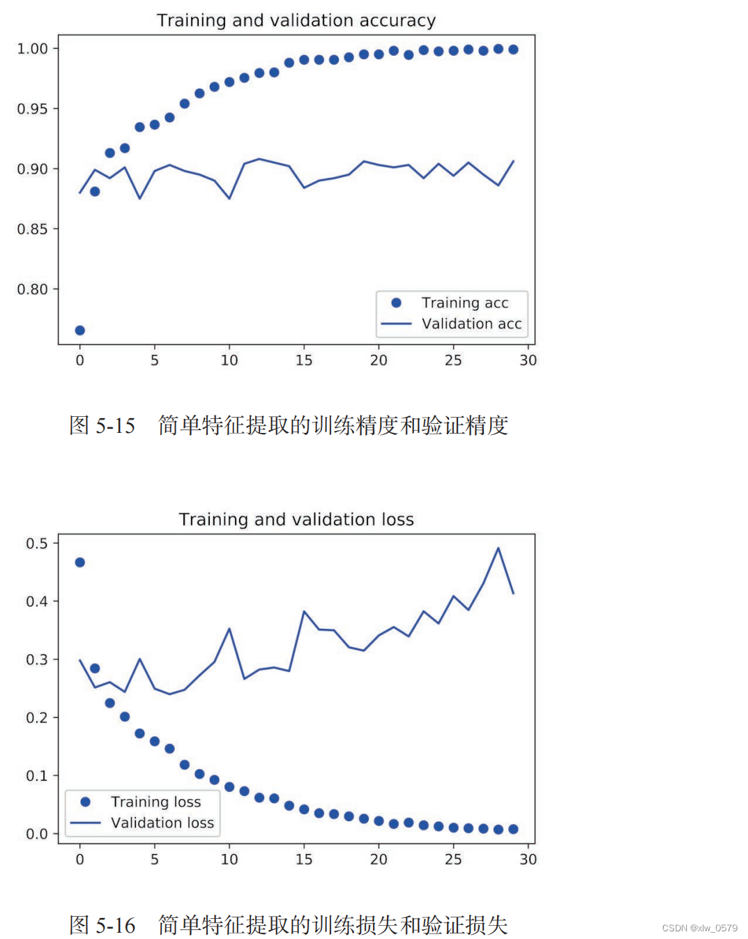
我们的验证精度达到了约 90%，比从头开始训练的小型模型效果要好得多。但从图中也可以看出，虽然 dropout 比率相当大，但模型几乎从一开始就过拟合。这是因为本方法没有使用数据增强，而数据增强对防止小型图像数据集的过拟合非常重要。

使用数据增强的特征提取

这种方法就是：扩展 conv_base 模型，然后在输入数据上端到端地运行模型。

from keras import models
from keras import layers
model = models.Sequential()
model.add(conv_base)
model.add(layers.Flatten())
model.add(layers.Dense(256, activation='relu'))
model.add(layers.Dense(1, activation='sigmoid'))

现在模型的架构如下所示

model.summary()
_________________________________________________________________
Layer (type)                 Output Shape              Param #   
=================================================================
vgg16 (Model)                (None, 4, 4, 512)         14714688  
_________________________________________________________________
flatten_1 (Flatten)          (None, 8192)              0         
_________________________________________________________________
dense_3 (Dense)              (None, 256)               2097408   
_________________________________________________________________
dense_4 (Dense)              (None, 1)                 257       
=================================================================
Total params: 16,812,353
Trainable params: 16,812,353
Non-trainable params: 0

VGG16 的卷积基有 14 714 688 个参数，非常多。在其上添加的分类器有 200 万个参数。
在编译和训练模型之前，一定要“冻结”卷积基。冻结（freeze）一个或多个层是指在训练过程中保持其权重不变。如果不这么做，那么卷积基之前学到的表示将会在训练过程中被修改。因为其上添加的 Dense 层是随机初始化的，所以非常大的权重更新将会在网络中传播，对之前学到的表示造成很大破坏。

 conv_base.trainable = False

如此设置之后，只有添加的两个 Dense 层的权重才会被训练。总共有 4 个权重张量，每层2 个（主权重矩阵和偏置向量）。
利用冻结的卷积基端到端地训练模型

from keras.preprocessing.image import ImageDataGenerator

train_datagen = ImageDataGenerator(
      rescale=1./255,
      rotation_range=40,
      width_shift_range=0.2,
      height_shift_range=0.2,
      shear_range=0.2,
      zoom_range=0.2,
      horizontal_flip=True,
      fill_mode='nearest')

# Note that the validation data should not be augmented!
test_datagen = ImageDataGenerator(rescale=1./255)

train_generator = train_datagen.flow_from_directory(
        # This is the target directory
        train_dir,
        # All images will be resized to 150x150
        target_size=(150, 150),
        batch_size=20,
        # Since we use binary_crossentropy loss, we need binary labels
        class_mode='binary')

validation_generator = test_datagen.flow_from_directory(
        validation_dir,
        target_size=(150, 150),
        batch_size=20,
        class_mode='binary')

model.compile(loss='binary_crossentropy',
              optimizer=optimizers.RMSprop(lr=2e-5),
              metrics=['acc'])

history = model.fit(
      train_generator,
      steps_per_epoch=100,
      epochs=30,
      validation_data=validation_generator,
      validation_steps=50,
      verbose=2)

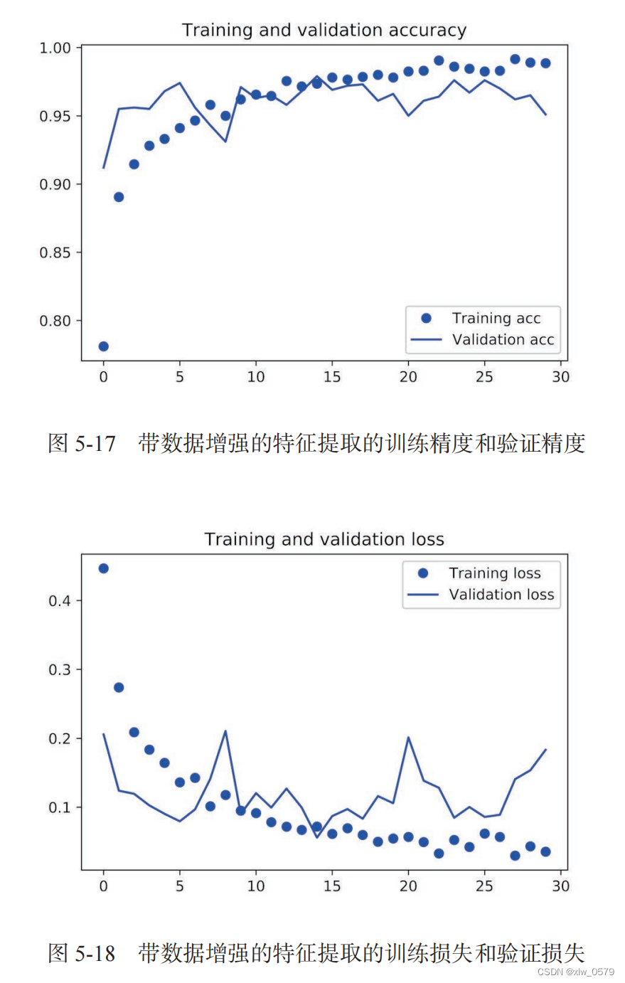
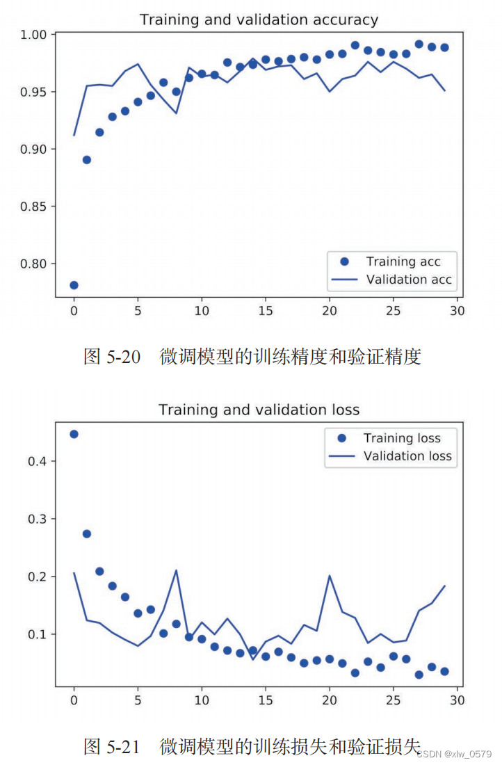
如你所见，验证精度约为 96%。这比从头开始训练的小型卷积神经网络要好得多。

微调模型

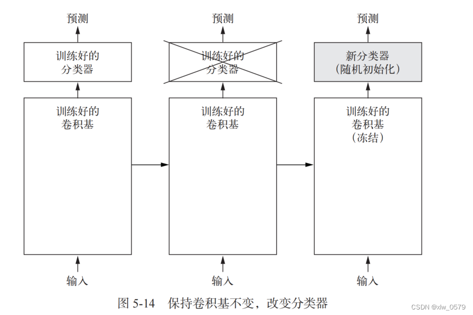
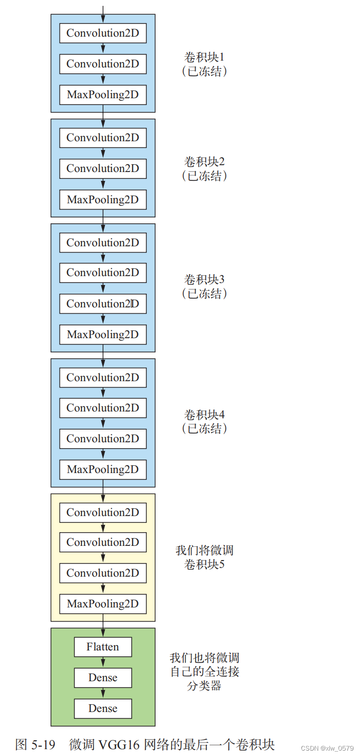
另一种广泛使用的模型复用方法是模型微调（fine-tuning），与特征提取互为补充。对于用于特征提取的冻结的模型基，微调是指将其顶部的几层“解冻”，并将这解冻的几层和新增加的部分（本例中是全连接分类器）联合训练（见图 5-19）。之所以叫作微调。

微调网络的步骤如下。
(1) 在已经训练好的基网络（base network）上添加自定义网络。
(2) 冻结基网络。
(3) 训练所添加的部分。
(4) 解冻基网络的一些层。
(5) 联合训练解冻的这些层和添加的部分。
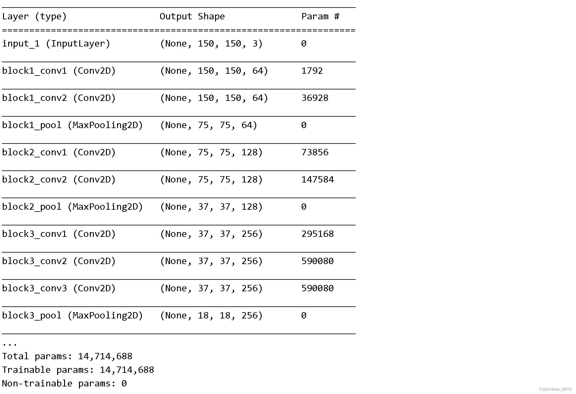
卷积基的架构如下所示。

conv_base.summary()
_________________________________________________________________
Layer (type) Output Shape Param # 
=================================================================
input_1 (InputLayer) (None, 150, 150, 3) 0 
_________________________________________________________________
block1_conv1 (Conv2D) (None, 150, 150, 64) 1792 
_________________________________________________________________
block1_conv2 (Conv2D) (None, 150, 150, 64) 36928 
_________________________________________________________________
block1_pool (MaxPooling2D) (None, 75, 75, 64) 0 
_________________________________________________________________
block2_conv1 (Conv2D) (None, 75, 75, 128) 73856 
_________________________________________________________________
block2_conv2 (Conv2D) (None, 75, 75, 128) 147584 
_________________________________________________________________
block2_pool (MaxPooling2D) (None, 37, 37, 128) 0 
_________________________________________________________________
block3_conv1 (Conv2D) (None, 37, 37, 256) 295168 
_________________________________________________________________
block3_conv2 (Conv2D) (None, 37, 37, 256) 590080 
_________________________________________________________________
block3_conv3 (Conv2D) (None, 37, 37, 256) 590080 
_________________________________________________________________
block3_pool (MaxPooling2D) (None, 18, 18, 256) 0 
_________________________________________________________________
block4_conv1 (Conv2D) (None, 18, 18, 512) 1180160 
_________________________________________________________________
block4_conv2 (Conv2D) (None, 18, 18, 512) 2359808 
_________________________________________________________________
block4_conv3 (Conv2D) (None, 18, 18, 512) 2359808 
_________________________________________________________________
block4_pool (MaxPooling2D) (None, 9, 9, 512) 0 
_________________________________________________________________
block5_conv1 (Conv2D) (None, 9, 9, 512) 2359808 
_________________________________________________________________
block5_conv2 (Conv2D) (None, 9, 9, 512) 2359808 
_________________________________________________________________
block5_conv3 (Conv2D) (None, 9, 9, 512) 2359808
_________________________________________________________________
block5_pool (MaxPooling2D) (None, 4, 4, 512) 0 
=================================================================
Total params: 14,714,688
Trainable params: 0
Non-trainable params: 14,714,688

我们将微调最后三个卷积层，也就是说，直到 block4_pool 的所有层都应该被冻结，而block5_conv1、block5_conv2 和 block5_conv3 三层应该是可训练的。
为什么不微调更多层？为什么不微调整个卷积基？你当然可以这么做，但需要考虑以下几点。

• 卷积基中更靠底部的层编码的是更加通用的可复用特征，而更靠顶部的层编码的是更专业化的特征。微调这些更专业化的特征更加有用，因为它们需要在你的新问题上改变用途。微调更靠底部的层，得到的回报会更少。
• 训练的参数越多，过拟合的风险越大。卷积基有 1500 万个参数，所以在你的小型数据集上训练这么多参数是有风险的。

冻结直到某一层的所有层

conv_base.trainable = True

set_trainable = False
for layer in conv_base.layers:
    if layer.name == 'block5_conv1':
        set_trainable = True
    if set_trainable:
        layer.trainable = True
    else:
        layer.trainable = False

微调模型

model.compile(loss='binary_crossentropy',
              optimizer=optimizers.RMSprop(lr=1e-5),
              metrics=['acc'])

history = model.fit(
      train_generator,
      steps_per_epoch=100,
      epochs=100,
      validation_data=validation_generator,
      validation_steps=50)