十、卷积神经网络的可视化1

人们常说，深度学习模型是“黑盒”，即模型学到的表示很难用人类可以理解的方式来提取和呈现。虽然对于某些类型的深度学习模型来说，这种说法部分正确，但对卷积神经网络来说绝对不是这样。卷积神经网络学到的表示非常适合可视化，很大程度上是因为它们是视觉概念
的表示。

• 可视化卷积神经网络的中间输出（中间激活）：有助于理解卷积神经网络连续的层如何对输入进行变换，也有助于初步了解卷积神经网络每个过滤器的含义。
• 可视化卷积神经网络的过滤器：有助于精确理解卷积神经网络中每个过滤器容易接受的视觉模式或视觉概念。
• 可视化图像中类激活的热力图：有助于理解图像的哪个部分被识别为属于某个类别，从而可以定位图像中的物体。

可视化中间激活，是指对于给定输入，展示网络中各个卷积层和池化层输出的特征图（层的输出通常被称为该层的激活，即激活函数的输出）。
首先来加载 保存的模型。

>>> from keras.models import load_model
>>> model = load_model('cats_and_dogs_small_2.h5')
>>> model.summary() # 作为提醒
_________________________________________________________________
Layer (type) Output Shape Param # 
=================================================================
conv2d_5 (Conv2D) (None, 148, 148, 32) 896 
_________________________________________________________________
max_pooling2d_5 (MaxPooling2D) (None, 74, 74, 32) 0 
_________________________________________________________________
conv2d_6 (Conv2D) (None, 72, 72, 64) 18496 
_________________________________________________________________
max_pooling2d_6 (MaxPooling2D) (None, 36, 36, 64) 0 
_________________________________________________________________
conv2d_7 (Conv2D) (None, 34, 34, 128) 73856 
_________________________________________________________________
max_pooling2d_7 (MaxPooling2D) (None, 17, 17, 128) 0 
_________________________________________________________________
conv2d_8 (Conv2D) (None, 15, 15, 128) 147584 
_________________________________________________________________
max_pooling2d_8 (MaxPooling2D) (None, 7, 7, 128) 0 
_________________________________________________________________
flatten_2 (Flatten) (None, 6272) 0 
_________________________________________________________________
dropout_1 (Dropout) (None, 6272) 0 
_________________________________________________________________
dense_3 (Dense) (None, 512) 3211776 
_________________________________________________________________
dense_4 (Dense) (None, 1) 513 
=================================================================
Total params: 3,453,121
Trainable params: 3,453,121
Non-trainable params: 0

输入图像

img_path = '/Users/fchollet/Downloads/cats_and_dogs_small/test/cats/cat.1700.jpg'
from keras.preprocessing import image 
import numpy as np
img = image.load_img(img_path, target_size=(150, 150)) 
img_tensor = image.img_to_array(img)
img_tensor = np.expand_dims(img_tensor, axis=0) 
img_tensor /= 255. 
# 其形状为 (1, 150, 150, 3)
print(img_tensor.shape)

为了提取想要查看的特征图，我们需要创建一个 Keras 模型，以图像批量作为输入，并输出所有卷积层和池化层的激活。为此，我们需要使用 Keras 的 Model 类。模型实例化需要两个参数：一个输入张量（或输入张量的列表）和一个输出张量（或输出张量的列表）。

from keras import models
layer_outputs = [layer.output for layer in model.layers[:8]] 
activation_model = models.Model(inputs=model.input, outputs=layer_outputs)

输入一张图像，这个模型将返回原始模型前 8 层的激活值。这是你在本书中第一次遇到的多输出模型，之前的模型都是只有一个输入和一个输出。一般情况下，模型可以有任意个输入和输出。这个模型有一个输入和 8 个输出，即每层激活对应一个输出。
以预测模式运行模型

activations = activation_model.predict(img_tensor)

对于输入的猫图像，第一个卷积层的激活如下所示。

>>> first_layer_activation = activations[0]
>>> print(first_layer_activation.shape)
(1, 148, 148, 32)

它是大小为 148×148 的特征图，有 32 个通道。我们来绘制原始模型第一层激活的第 4 个通道

import matplotlib.pyplot as plt
plt.matshow(first_layer_activation[0, :, :, 4], cmap='viridis')

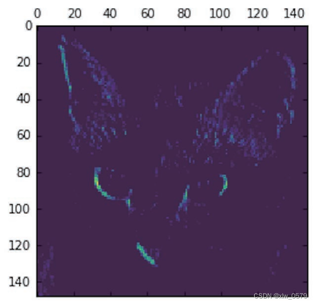
这个通道似乎是对角边缘检测器。
我们再看一下第 7 个通道（见图 5-26）。但请注意，你的通道可能与此不同，因为卷积层学到的过滤器并不是确定的。

plt.matshow(first_layer_activation[0, :, :, 7], cmap='viridis'

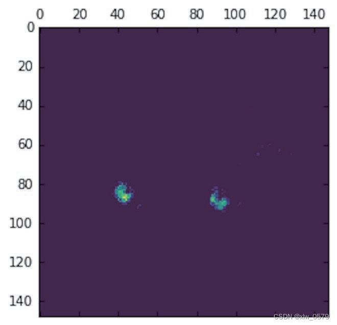
这个通道看起来像是“鲜绿色圆点”检测器，对寻找猫眼睛很有用。
将每个中间激活的所有通道可视化

import keras

# These are the names of the layers, so can have them as part of our plot
layer_names = []
for layer in model.layers[:8]:
    layer_names.append(layer.name)

images_per_row = 16

# Now let's display our feature maps
for layer_name, layer_activation in zip(layer_names, activations):
    # This is the number of features in the feature map
    n_features = layer_activation.shape[-1]

    # The feature map has shape (1, size, size, n_features)
    size = layer_activation.shape[1]

    # We will tile the activation channels in this matrix
    n_cols = n_features // images_per_row
    display_grid = np.zeros((size * n_cols, images_per_row * size))

    # We'll tile each filter into this big horizontal grid
    for col in range(n_cols):
        for row in range(images_per_row):
            channel_image = layer_activation[0,
                                             :, :,
                                             col * images_per_row + row]
            # Post-process the feature to make it visually palatable
            channel_image -= channel_image.mean()
            channel_image /= channel_image.std()
            channel_image *= 64
            channel_image += 128
            channel_image = np.clip(channel_image, 0, 255).astype('uint8')
            display_grid[col * size : (col + 1) * size,
                         row * size : (row + 1) * size] = channel_image

    # Display the grid
    scale = 1. / size
    plt.figure(figsize=(scale * display_grid.shape[1],
                        scale * display_grid.shape[0]))
    plt.title(layer_name)
    plt.grid(False)
    plt.imshow(display_grid, aspect='auto', cmap='viridis')
    
plt.show()

• 第一层是各种边缘探测器的集合。在这一阶段，激活几乎保留了原始图像中的所有信息。
• 随着层数的加深，激活变得越来越抽象，并且越来越难以直观地理解。它们开始表示更高层次的概念，比如“猫耳朵”和“猫眼睛”。层数越深，其表示中关于图像视觉内容的信息就越少，而关于类别的信息就越多。
• 激活的稀疏度（sparsity）随着层数的加深而增大。在第一层里，所有过滤器都被输入图像激活，但在后面的层里，越来越多的过滤器是空白的。也就是说，输入图像中找不到这些过滤器所编码的模式。

我们刚刚揭示了深度神经网络学到的表示的一个重要普遍特征：随着层数的加深，层所提取的特征变得越来越抽象。更高的层激活包含关于特定输入的信息越来越少，而关于目标的信息越来越多（本例中即图像的类别：猫或狗）。深度神经网络可以有效地作为信息蒸馏管道（information distillation pipeline），输入原始数据（本例中是 RGB 图像），反复对其进行变换，将无关信息过滤掉（比如图像的具体外观），并放大和细化有用的信息（比如图像的类别）。这与人类和动物感知世界的方式类似：人类观察一个场景几秒钟后，可以记住其中有哪些抽象物体（比如自行车、树），但记不住这些物体的具体外观。事实上，如果你试着凭记忆画一辆普通自行车，那么很可能完全画不出真实的样子，虽然你一生中见过上千辆自行车。你可以现在就试着画一下，这个说法绝对是真实的。你的大脑已经学会将视觉输入完全抽象化，即将其转换为更高层次的视觉概念，同时过滤掉不相关的视觉细节，这使得大脑很难记住周围事物的外观。