【AI大模型实践教程】如何利用大模型简化开发过程提高开发效率？

史蒂夫・乔布斯曾经把计算机称作 “心灵之自行车”。不过，人们对他这个比喻的背景知之甚少，他是在谈及地球上所有物种移动效率的时候提到的。

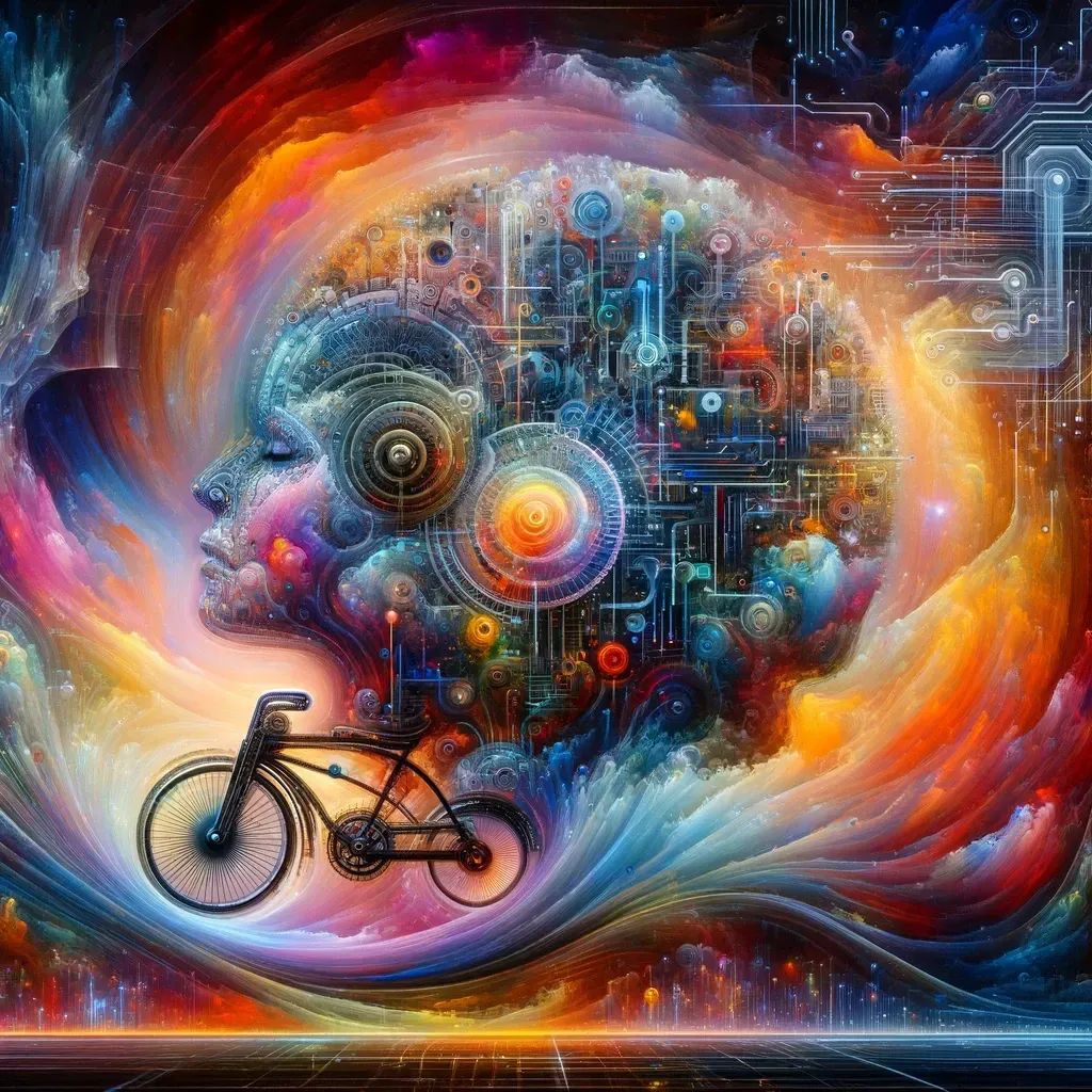
由 DALL·E 3 生成的图片，提示 “将计算机想象成心灵的自行车”

秃鹫赢了，位居榜首，超过了其他所有物种。人类排在榜单大约三分之一的位置…… 但是，一旦人类骑上自行车，就能远远超越秃鹫，登顶榜首。这让我深受启发，人类是工具制造者，我们可以制造出将这些固有能力放大到惊人程度的工具。对我来说，计算机一直是思维的自行车，它让我们远远超越了固有的能力。我认为我们只是处于这个工具的早期阶段，非常早期的阶段。我们只走了很短的一段距离，它仍处于形成阶段，但我们已经看到了巨大的变化。我认为，与未来 100 年发生的事情相比，这算不了什么。

—— 史蒂夫・乔布斯（1990）

#01

谨慎乐观

LLM 在加速软件开发方面的作用引发了广泛讨论。有人认为，自动生成的代码质量过低，以至于使用这些代码产生的是负面效果。而另一方面，许多人声称编程的时代已经结束。已经有众多研究试图客观评估 LLM 在诸如 HumanEval 或 MBPP 这样的代码质量基准数据集上的表现。这些评估对于该领域的发展至关重要，但这并非本文的焦点。

本文旨在为开发者，尤其是那些对利用这些模型持保留态度的开发者，提供实用的建议。要注意的是，我相信通过恰当地使用这项技术，一个人的工作效率确实能够实现质的飞跃。

需要明确的是，使用 LLM 并不意味着一定能产出高性能的代码。即便是最先进的模型也会犯下严重的错误。但重要的是要记住，最优秀的人类工程师也难免犯错。这就是我们为什么不会在没有设置防护措施的情况下发布代码，比如进行自动化测试和同行评审。LLM 没有改变最佳实践的本质，但可能改变了实现这些最佳实践的容易度。

描述现在交付代码的过程（图片由 DALL·E 3 生成）

编写高性能代码的速度真的那么重要吗？

如果大多数专业软件工程师的大部分时间都花在了键盘敲击上，我会觉得非常意外。如果真是这样，我们或许会更认真地把 “代码行数” 当作衡量工作表现的一个标准。**我认为，工程师实际上更多的时间是用来决定首先需要编写哪些代码。**目前，LLM 还没有能力进行这种高级的抽象思维 ——OpenAI 和许多其他机构正在努力使这些步骤成为可能，但这很可能需要的不仅仅是增加模型的参数或扩大训练数据，而是需要一种全新的思维方式。然而，LLM 已经能够在很大程度上加速我们的工作中的很大一部分了。

#02

编写高效的函数

让我举个例子来说明，当 LLM 生成了一小段代码后，我们需要采取哪些步骤来优化它，使之变得实用。在地球上的某个点和另一组坐标之间测量距离是地理信息分析中的一个常见任务。想象一下这样的情境。

首先看到的代码输出是这样的：

import math  
  
def haversine(lat1, lon1, lat2, lon2):  
    # Radius of the Earth in kilometers  
    R = 6371.0  
  
    # Convert degrees to radians  
    lat1\_rad = math.radians(lat1)  
    lon1\_rad = math.radians(lon1)  
    lat2\_rad = math.radians(lat2)  
    lon2\_rad = math.radians(lon2)  
  
    # Differences in coordinates  
    dlat = lat2\_rad - lat1\_rad  
    dlon = lon2\_rad - lon1\_rad  
  
    # Haversine formula  
    a = math.sin(dlat / 2)\*\*2 + math.cos(lat1\_rad) \* math.cos(lat2\_rad) \* math.sin(dlon / 2)\*\*2  
    c = 2 \* math.atan2(math.sqrt(a), math.sqrt(1 - a))  
  
    # Distance in kilometers  
    distance = R \* c  
  
    return distance  
  
def find\_closest\_oil\_platform(vessel\_lat, vessel\_lon, platforms):  
    closest\_platform = None  
    min\_distance = float('inf')  
      
    for platform in platforms:  
        distance = haversine(vessel\_lat, vessel\_lon, platform\['latitude'\], platform\['longitude'\])  
        if distance < min\_distance:  
            min\_distance = distance  
            closest\_platform = platform  
  
    return closest\_platform, min\_distance

那么，这段代码的质量怎么样呢？

这段代码的质量并不理想。它的问题不少，最明显的是它难以阅读，因为它使用了难以理解和不一致的变量命名，包括大小写的单字符命名。此外，它缺少了文档说明和类型提示，使用了一个不必要且低效的 for 循环，也没有处理一些特殊情况，比如相等距离的问题。

但经过修改之后：

from typing import Tuple, List  
import numpy as np  
  
def haversine\_vectorized(vessel\_lat: float, vessel\_lon: float, platform\_lats: np.ndarray, platform\_lons: np.ndarray) -> np.ndarray:  
    """  
    Calculate the Haversine distance between a vessel and multiple platforms in a vectorized manner.  
  
    Parameters:  
    - vessel\_lat: Latitude of the vessel in decimal degrees.  
    - vessel\_lon: Longitude of the vessel in decimal degrees.  
    - platform\_lats: Numpy array of latitudes of oil platforms in decimal degrees.  
    - platform\_lons: Numpy array of longitudes of oil platforms in decimal degrees.  
  
    Returns:  
    - distances: Numpy array of distances from the vessel to each platform in kilometers.  
    """  
    # Convert decimal degrees to radians  
    lat1, lon1, lat2, lon2 = map(np.radians, \[vessel\_lat, vessel\_lon, platform\_lats, platform\_lons\])  
  
    # Haversine formula  
    dlat = lat2 - lat1  
    dlon = lon2 - lon1  
    a = np.sin(dlat/2)\*\*2 + np.cos(lat1) \* np.cos(lat2) \* np.sin(dlon/2)\*\*2  
    c = 2 \* np.arctan2(np.sqrt(a), np.sqrt(1\-a))  
    r = 6371  # Radius of Earth in kilometers  
    return c \* r  
  
def find\_closest\_platform(vessel\_lat: float, vessel\_lon: float, platform\_lats: np.ndarray, platform\_lons: np.ndarray) -> Tuple\[List\[int\], float\]:  
    """  
    Finds the closest oil platform(s) to a vessel given arrays of platform latitudes and longitudes, handling equidistant platforms.  
  
    Parameters:  
    - vessel\_lat: Latitude of the vessel in decimal degrees.  
    - vessel\_lon: Longitude of the vessel in decimal degrees.  
    - platform\_lats: Numpy array of latitudes for oil platforms.  
    - platform\_lons: Numpy array of longitudes for oil platforms.  
  
    Returns:  
    - A tuple containing a list of indices of the closest platforms and the distance to them in kilometers.  
    """  
    # Calculate distances to all platforms  
    distances = haversine\_vectorized(vessel\_lat, vessel\_lon, platform\_lats, platform\_lons)  
      
    # Find the minimum distance  
    min\_distance = np.min(distances)  
      
    # Find all indices with the minimum distance  
    closest\_indices = np.where(distances == min\_distance)\[0\].tolist()  
  
    # Return the indices of all closest platforms and the minimum distance  
    return closest\_indices, min\_distance

改进后的代码有了明显提升。它变得更容易阅读了，增加了文档说明和类型提示，并且用更高效的向量计算方式替换了原有的 for 循环。

但是，代码的 “好坏”，更重要的是，它是否满足需求这些都取决于代码将要运行的具体环境。要知道，我们无法仅凭几行代码就能有效评估其质量，这一点对人类如此，对 LLM 也是如此。

比如说，这段代码的准确度是否满足用户的预期？它会被频繁运行吗？是一年一次，还是每微秒一次？使用的硬件条件如何？预期的使用量和规模是否值得我们去追求那些细小的优化？在考虑到你的薪资之后，这样做是否划算？

让我们在上述因素的基础上来评估这段代码。

在准确性方面，虽然半正矢公式（haversine formula）表现不错，但并非最佳选择，因为它将地球视为一个完美的球体，而实际上地球更接近于一个扁球体。在需要跨越巨大距离进行毫米级精确测量时，这种差异变得非常重要。如果真的需要这样的精确度，虽然有更精确的公式（如 Vincenty 公式）可用，但这会带来性能上的折中。因为对于这段代码的用户而言，毫米级的精确度并不是必须的（事实上，由于卫星图像导出的船舶坐标的误差，这种精度也并不相关），所以在准确性方面，半正弦函数是一个合理的选择。

代码运行得够快吗？考虑到只需要对几千个海上石油平台计算距离，特别是通过向量计算方法，这种计算是非常高效的。但如果应用场景变成了计算与岸边任意点的距离（岸线上有数以亿计的点），那么采用 “分而治之” 的策略可能会更加合适。在实际应用中，考虑到节约计算成本的需要，这个函数设计为在一个尽可能配置低的虚拟机上每天运行约 1 亿次。

基于这些详细的背景信息，我们可以认为上面的代码实现是合理的。这也意味着，在代码最终合并前，它应该先经过测试（我通常不推荐仅依赖 LLM 进行测试）和人工同行评审。

#03

加速前进

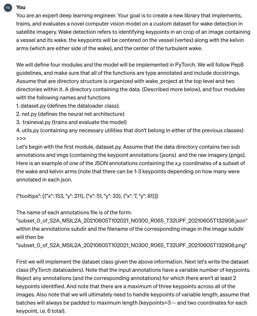
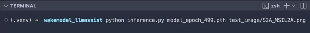
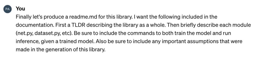
像之前那样利用 LLM 自动生成实用的函数不仅可以节省时间，而且当你开始利用它们来生成整套的库、处理模块间的依赖、撰写文档、实现可视化（通过多模态能力）、编写 README 文件、开发命令行接口等时，它们带来的价值将会成倍增长。

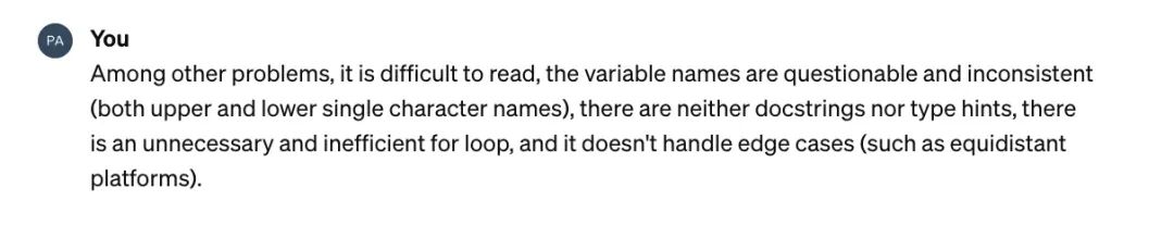
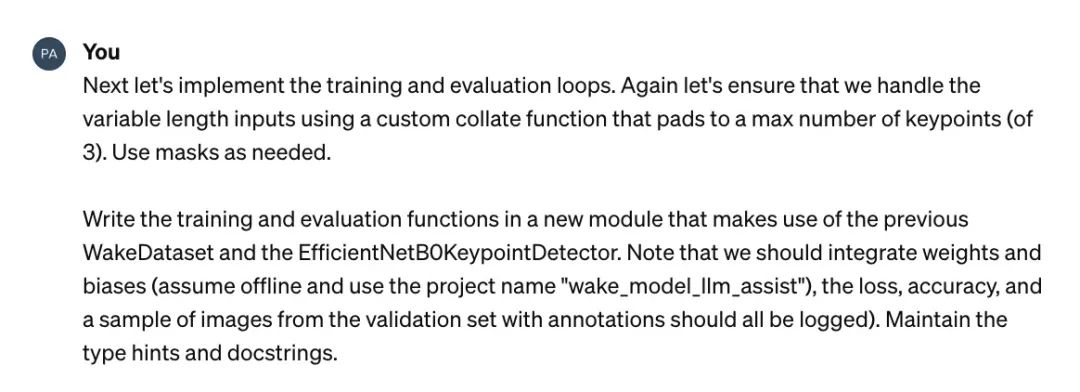
我们来试着从零开始，借助 LLM 的广泛辅助，创建、训练、评估并推断一个全新的计算机视觉模型。以一篇最近发表的论文为例，“通过深度学习识别 Sentinel-2 图像中船舶尾迹组件的关键点方法”（Del Prete 等人，IEEE GRSL，2023），这篇论文就是我们前进的动力和灵感来源。

论文链接：https://www.semanticscholar.org/paper/Keypoints-Method-for-Recognition-of-Ship-Wake-in-by-Prete-Graziano/a38d19b5ebaa2441e1bef2af0ecf24332bd6ca5b

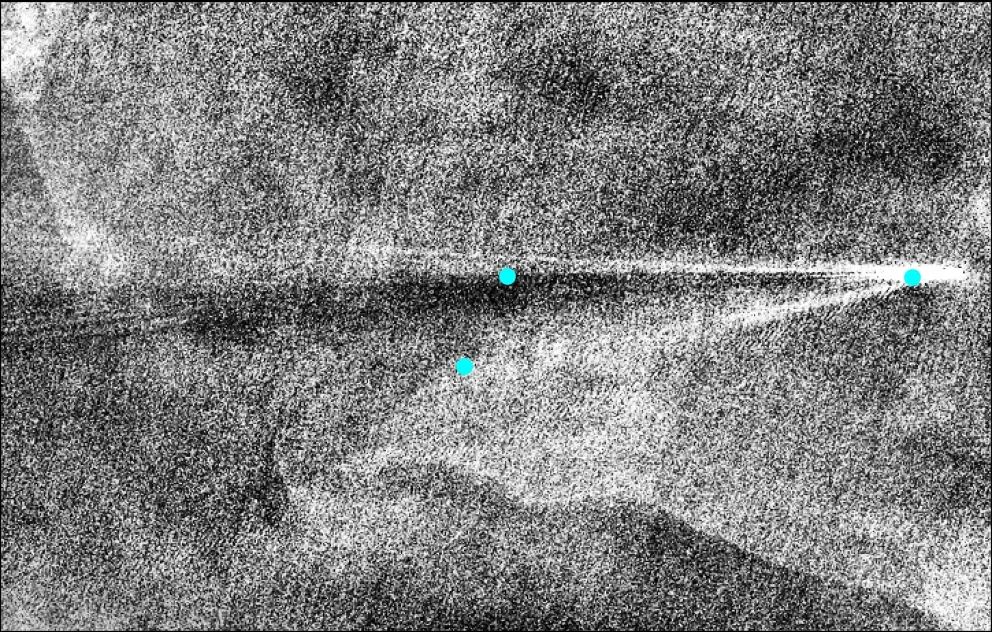
Sentinel-2 卫星图像中显示的一艘船及其尾流。

为什么我们需要关心船舶在卫星图像中的行进方向，这项任务有什么难点呢？

通过静态图像识别船只的航行方向，对于那些需要监控水域中人类活动的组织来说，是极其宝贵的信息。比如，如果一艘船正朝向一个海洋保护区行进，这可能意味着需要警觉或者采取拦截措施。通常，全球范围内公开的卫星图像的分辨率不足以精确判断一艘船的朝向，尤其是那些在图像上只占据几个像素的小型船只（例如，Sentinel-2 的图像分辨率为 10 米 / 像素）。然而，即便是小型船只留下的水波纹也可能相当明显，这就为我们提供了一个判断船只朝向和行进方向的线索，即使船的尾部无法直接识别。

这项研究之所以引人注目，是因为它采用的模型基于 EfficientNetB0，这是一个足够小的模型，能够在不花费太多计算资源的情况下进行大规模应用。虽然我没有找到具体的代码实现，但作者公开了包括标注在内的数据集，这是值得赞赏的一步。

https://zenodo.org/records/7947694

开始我们的探索吧！

如同启动任何新的机器学习项目一样，首先对数据进行可视化是极富启发性的一步。

import os  
import json  
from PIL import Image, ImageDraw  
import matplotlib.pyplot as plt  
import seaborn as sns  
  
# Define the path to your data directory  
data\_dir = "/path/to/your/data"  # Adjust this to the path of your data directory  
annotations\_dir = os.path.join(data\_dir, "annotations")  
images\_dir = os.path.join(data\_dir, "imgs")  
  
# Initialize Seaborn for better visual aesthetics  
sns.set(style="whitegrid", palette="muted")  
  
# Create a list to hold file paths for images and their corresponding annotations  
image\_files = \[\]  
annotation\_files = \[\]  
  
# Loop through the annotations directory to get the list of annotation files  
for annotation\_file in os.listdir(annotations\_dir):  
    if annotation\_file.endswith(".json"):  
        annotation\_path = os.path.join(annotations\_dir, annotation\_file)  
        image\_file = annotation\_file.replace(".json", ".png")  # Assuming image file names match annotation file names  
        image\_path = os.path.join(images\_dir, image\_file)  
  
        # Check if the corresponding image file exists  
        if os.path.exists(image\_path):  
            annotation\_files.append(annotation\_path)  
            image\_files.append(image\_path)  
  
# Plotting  
num\_examples = min(len(image\_files), 10)  # Limiting to 10 examples for visualization  
fig, axes = plt.subplots(2, 5, figsize=(20, 8))  
  
for idx, (image\_path, annotation\_path) in enumerate(zip(image\_files\[:num\_examples\], annotation\_files\[:num\_examples\])):  
    # Load the image  
    img = Image.open(image\_path).convert("RGB")  # Ensure the image is treated as RGB  
    draw = ImageDraw.Draw(img)  
  
    # Load the corresponding annotations and draw keypoints  
    with open(annotation\_path, 'r') as f:  
        annotations = json.load(f)  
        for point in annotations\["tooltips"\]:  
            x, y = point\["x"\], point\["y"\]  
            # Draw keypoints in cyan for visibility  
            draw.ellipse(\[(x-10, y-10), (x+10, y+10)\], fill='cyan', outline='black')  
  
    # Plot the image with keypoints  
    ax = axes\[idx // 5, idx % 5\]  
    ax.imshow(img)  
    ax.axis('off')  
    ax.set\_title(f"Image {idx+1}")  
  
plt.tight\_layout()  
plt.show()

结果如下：

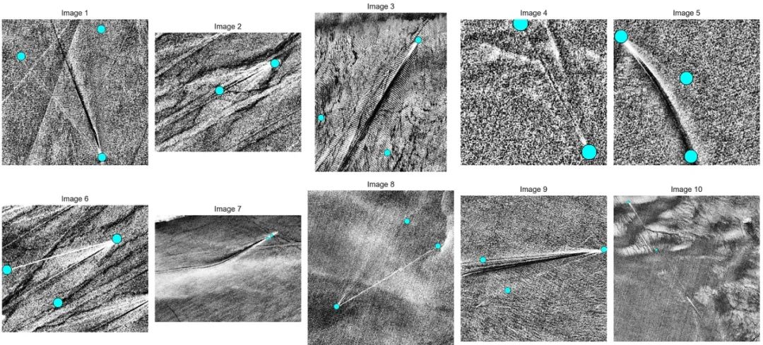Sentinel-2 卫星图像中的船只和尾流关键点注释（青色）样本。

结果展示了几个关键的发现：首先，不同图片中标注的关键点（青色点）数量不一；其次，这些图像都是灰度的，并且形状各异；第三，尽管样本量不大，但其内部差异性却相当大。在明确了这些基础之后，我们接下来将编写用于加载数据集、定义神经网络、进行训练和验证的代码。在请求代码之前，我们会先向 LLM 提供一些背景信息。

这导致了以下输出：

import os  
import json  
import torch  
from torch.utils.data import Dataset, DataLoader  
from torchvision import transforms  
from torchvision.io import read\_image  
from typing import Tuple, List  
  
class WakeDataset(Dataset):  
    """  
    Custom Dataset for loading wake detection imagery and annotations, with preprocessing for EfficientNet.  
    Images are grayscale and will be converted to three-channel images for model compatibility.  
    """  
      
    def \_\_init\_\_(self, annotations\_dir: str, images\_dir: str, transform=None):  
        """  
        Initializes the dataset with paths to annotations and images directories, and a transform.  
  
        Parameters:  
        - annotations\_dir: Path to the directory containing annotation JSON files.  
        - images\_dir: Path to the directory containing grayscale image files.  
        - transform: A torchvision.transforms transform to be applied on a sample.  
        """  
        self.annotations\_dir = annotations\_dir  
        self.images\_dir = images\_dir  
        self.transform = transform if transform else self.default\_transform()  
        self.annotations = self.\_load\_annotations()  
  
    def default\_transform(self):  
        """  
        Defines the default transform to resize images, convert them to three-channel format, and to tensors.  
  
        Returns:  
        - A torchvision.transforms composition for image preprocessing.  
        """  
        return transforms.Compose(\[  
            transforms.Resize((224, 224)),  # Resize to the input size for EfficientNet  
            transforms.Grayscale(num\_output\_channels=3),  # Convert grayscale to three-channel  
            transforms.ConvertImageDtype(torch.float),  # Ensures image is a float tensor  
        \])  
  
    def \_load\_annotations(self) -> List\[Tuple\[str, List\[int\]\]\]:  
        """  
        Loads and filters annotations with at least 2 keypoints.  
  
        Returns:  
        - A list of tuples, where each tuple contains the image filename and its keypoints.  
        """  
        annotations = \[\]  
        for filename in os.listdir(self.annotations\_dir):  
            if not filename.endswith('.json'):  
                continue  
            filepath = os.path.join(self.annotations\_dir, filename)  
            with open(filepath, 'r') as f:  
                data = json.load(f)  
                if len(data\['tooltips'\]) >= 2:  # Filter annotations with at least 2 keypoints  
                    keypoints = \[item for sublist in \[\[kp\['x'\], kp\['y'\]\] for kp in data\['tooltips'\]\] for item in sublist\]  
                    annotations.append((filename.replace('.json', '.png'), keypoints))  
        return annotations  
  
    def \_\_len\_\_(self) -> int:  
        """  
        Returns the number of items in the dataset.  
        """  
        return len(self.annotations)  
  
    def \_\_getitem\_\_(self, idx) -> Tuple\[torch.Tensor, torch.Tensor\]:  
        """  
        Retrieves an item from the dataset at the specified index, with preprocessing for EfficientNet.  
  
        Parameters:  
        - idx: Index of the item to retrieve.  
  
        Returns:  
        - A tuple containing the preprocessed image tensor and its corresponding keypoints tensor.  
        """  
        img\_name, keypoints = self.annotations\[idx\]  
        img\_path = os.path.join(self.images\_dir, img\_name)  
        image = read\_image(img\_path)  # Load image  
        keypoints = torch.tensor(keypoints + \[0\] \* (6 - len(keypoints)), dtype=torch.float)  # Pad keypoints  
        if self.transform:  
            image = self.transform(image)  
        return image, keypoints

最终得到的代码看起来还算合理，并且似乎注意到了问题的一些细节。虽然不是完美的（例如，选择在 default_transform 中将图像从灰度转为 RGB 颜色模式是个奇怪的决定，我个人更倾向于使用 pathlib 而非 os。listdir），但我们现在可以先放下这些细节不谈。

import torch  
import torch.nn as nn  
from torchvision import models  
from typing import Tuple  
  
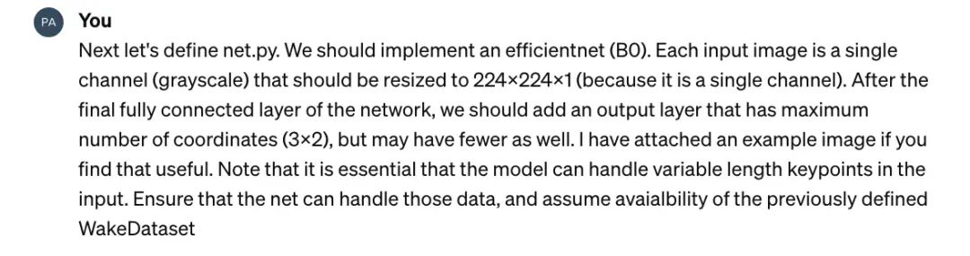
class EfficientNetB0KeypointDetector(nn.Module):  
    """  
    A custom EfficientNet-B0 model for keypoint detection in grayscale images.  
    The network modifies the input layer to accept single-channel images and   
    adds a custom output layer for predicting a fixed number of keypoints.  
    """  
  
    def \_\_init\_\_(self, num\_keypoints: int = 3):  
        """  
        Initializes the model.  
  
        Parameters:  
        - num\_keypoints: The number of keypoints to predict. Default is 3,   
                         corresponding to the maximum number of keypoints in the dataset.  
        """  
        super(EfficientNetB0KeypointDetector, self).\_\_init\_\_()  
        self.num\_keypoints = num\_keypoints  
        # Load a pre-trained EfficientNet-B0  
        self.efficientnet\_b0 = models.efficientnet\_b0(pretrained=True)  
          
        # Modify the first convolutional layer to accept single-channel (grayscale) images  
        original\_first\_conv = self.efficientnet\_b0.features\[0\]\[0\]  
        self.efficientnet\_b0.features\[0\]\[0\] = nn.Conv2d(  
            in\_channels=1,   
            out\_channels=original\_first\_conv.out\_channels,   
            kernel\_size=original\_first\_conv.kernel\_size,   
            stride=original\_first\_conv.stride,   
            padding=original\_first\_conv.padding,   
            bias=False)  
  
        # Modify the classifier to predict keypoints (num\_keypoints \* 2 because x, y for each keypoint)  
        self.efficientnet\_b0.classifier = nn.Linear(  
            in\_features=self.efficientnet\_b0.classifier\[1\].in\_features,   
            out\_features=num\_keypoints \* 2)  
  
    def forward(self, x: torch.Tensor) -> torch.Tensor:  
        """  
        Forward pass of the network.  
  
        Parameters:  
        - x: Input tensor of shape (batch\_size, 1, 224, 224)  
  
        Returns:  
        - A tensor of shape (batch\_size, num\_keypoints \* 2) representing the predicted keypoints.  
        """  
        return self.efficientnet\_b0(x)  
  
# Example usage  
if \_\_name\_\_ == "\_\_main\_\_":  
    model = EfficientNetB0KeypointDetector()  
    print(model)  
  
    # Example input tensor (batch\_size, channels, height, width)  
    example\_input = torch.randn(1, 1, 224, 224)  
    output = model(example\_input)  
    print(output.shape)  # Expected shape: (1, 6) for 3 keypoints (each with x, y coordinates)

import os  
import torch  
import torch.nn as nn  
import torch.optim as optim  
from torch.utils.data import DataLoader  
from dataset import WakeDataset, get\_dataloader  # Assuming dataset.py is in the same directory  
from net import EfficientNetB0KeypointDetector  
from torchvision import transforms  
import wandb  
  
# Initialize Weights & Biases  
wandb.init(project="wake\_model\_llm\_assist", entity="your\_wandb\_entity", mode="offline")  
  
def custom\_collate\_fn(batch):  
    """  
    Custom collate function to pad keypoints to a fixed size.  
      
    Parameters:  
    - batch: A list of tuples (image, keypoints).  
      
    Returns:  
    - Batched images and keypoints with padding as necessary.  
    """  
    images, keypoints = zip(\*batch)  
    images = torch.stack(images, 0)  
    max\_keypoints = 3 \* 2  # Maximum number of keypoints (3) times 2 for (x, y)  
    padded\_keypoints = \[torch.cat((kp, torch.zeros(max\_keypoints - len(kp)))) for kp in keypoints\]  
    keypoints = torch.stack(padded\_keypoints, 0)  
    return images, keypoints  
  
def train\_one\_epoch(model: nn.Module, dataloader: DataLoader, optimizer: optim.Optimizer, device: torch.device):  
    """  
    Trains the model for one epoch.  
      
    Parameters:  
    - model: The neural network model.  
    - dataloader: DataLoader providing the training data.  
    - optimizer: Optimizer used for model training.  
    - device: The device to train on.  
    """  
    model.train()  
    total\_loss = 0.0  
    for images, keypoints in dataloader:  
        images, keypoints = images.to(device), keypoints.to(device)  
        optimizer.zero\_grad()  
        outputs = model(images)  
        loss = nn.MSELoss()(outputs, keypoints)  
        loss.backward()  
        optimizer.step()  
        total\_loss += loss.item()  
      
    average\_loss = total\_loss / len(dataloader)  
    wandb.log({"train\_loss": average\_loss})  
  
def evaluate(model: nn.Module, dataloader: DataLoader, device: torch.device):  
    """  
    Evaluates the model on the validation set.  
      
    Parameters:  
    - model: The neural network model.  
    - dataloader: DataLoader providing the validation data.  
    - device: The device to evaluate on.  
    """  
    model.eval()  
    total\_loss = 0.0  
    with torch.no\_grad():  
        for images, keypoints in dataloader:  
            images, keypoints = images.to(device), keypoints.to(device)  
            outputs = model(images)  
            loss = nn.MSELoss()(outputs, keypoints)  
            total\_loss += loss.item()  
      
    average\_loss = total\_loss / len(dataloader)  
    wandb.log({"val\_loss": average\_loss})  
  
def main():  
    # Setup  
    device = torch.device("cuda" if torch.cuda.is\_available() else "cpu")  
    model = EfficientNetB0KeypointDetector().to(device)  
    optimizer = optim.Adam(model.parameters(), lr=1e-3)  
  
    # DataLoaders  
    train\_dataloader = get\_dataloader('path/to/train/annotations', 'path/to/train/images', batch\_size=4, transform=transforms.ToTensor(), collate\_fn=custom\_collate\_fn)  
    val\_dataloader = get\_dataloader('path/to/val/annotations', 'path/to/val/images', batch\_size=4, transform=transforms.ToTensor(), collate\_fn=custom\_collate\_fn)  
  
    # Training loop  
    for epoch in range(num\_epochs):  
        train\_one\_epoch(model, train\_dataloader, optimizer, device)  
        evaluate(model, val\_dataloader, device)  
        # Log model checkpoints, images, or other metrics as needed  
        wandb.log({})  
  
if \_\_name\_\_ == "\_\_main\_\_":  
    main()  

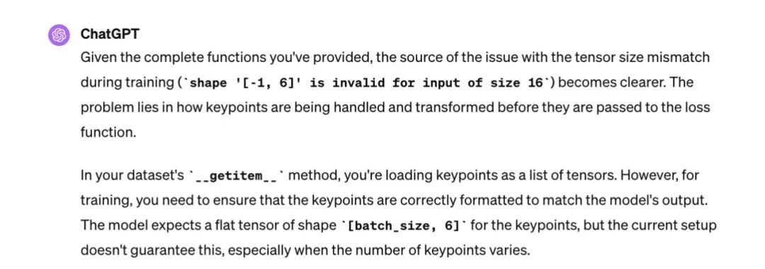
当我开始尝试运行代码时，遇到了一系列与张量形状不匹配相关的问题（想起了之前 RGB 与灰度图像的差异以及自定义 collate 函数的问题）。我尝试了几分钟的调试，但最终选择将所有模块代码复制到提示框里，让它帮我一起找出问题所在。

这样做有效解决了所有挂起的问题，我随即开始了模型的训练…… 但训练速度慢得出奇。这时我才意识到我没有利用 Apple 芯片上的 Metal 性能着色器（MPS）后端。虽然我平时不太在个人电脑上训练模型，MPS 对我还比较新，但我还是决定添加一个条件判断来使用它。

鉴于训练数据量适中（共 581 张图片），加上 EfficientNet 已经在 ImageNet 上进行了预训练，我决定进行 1000 个周期的训练。

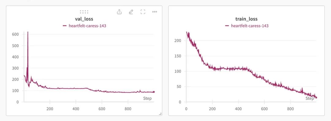
500 个周期后，train_loss 仍在减少，但验证损失似乎已经收敛（至少对于快速评估而言足够收敛）。图像是根据权重和偏差复制的。

值得注意的是，尽管存在一些已经在卫星图像上进行预训练的基础模型（相对于 ImageNet），这些模型很可能对这项任务更有效，但这些网络体积比 EfficientNet 大得多，因此训练速度更慢（而且太新，还没被 LLM 训练数据集包括）。

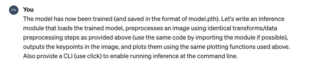
现在，让我们编写一个推理脚本和一个命令行界面（CLI），来测试我们刚训练好的模型。

import torch  
from torchvision import transforms  
from PIL import Image  
import matplotlib.pyplot as plt  
import click  
  
# Assuming net.py contains the EfficientNetB0KeypointDetector class  
# and dataset.py contains the transforms used during training  
from net import EfficientNetB0KeypointDetector  
from dataset import WakeDataset  # Modify as necessary to import transforms  
  
def load\_model(model\_path):  
    """Load the trained model from a file."""  
    model = EfficientNetB0KeypointDetector()  
    model.load\_state\_dict(torch.load(model\_path))  
    model.eval()  # Set the model to inference mode  
    return model  
  
def preprocess\_image(image\_path, transform):  
    """Load and preprocess an image."""  
    image = Image.open(image\_path).convert("L")  # Assuming grayscale conversion as in your dataset  
    image = transform(image)  
    # Add batch dimension (BxCxHxW)  
    image = image.unsqueeze(0)  
    return image  
  
def plot\_keypoints(image, keypoints):  
    """Plot keypoints on the image."""  
    plt.imshow(image.squeeze(), cmap='gray')  # Remove batch dimension and show image  
    plt.scatter(keypoints\[:, 0\], keypoints\[:, 1\], s=50, marker='.', c='red')  
    plt.show()  
  
@click.command()  
@click.argument('model\_path', type\=click.Path(exists=True))  
@click.argument('image\_path', type\=click.Path(exists=True))  
def run\_inference(model\_path, image\_path):  
    """Run inference on an image using a trained model."""  
    # Use the same transforms as during training  
    transform = transforms.Compose(\[  
        transforms.Resize((224, 224)),  
        transforms.ToTensor(),  
        transforms.Grayscale(num\_output\_channels=3),  
    \])  
      
    model = load\_model(model\_path)  
    image = preprocess\_image(image\_path, transform)  
      
    # Perform inference  
    with torch.no\_grad():  
        keypoints = model(image)  
        keypoints = keypoints.view(-1, 2).cpu().numpy()  # Reshape and convert to numpy for plotting  
      
    # Load original image for plotting  
    original\_image = Image.open(image\_path).convert("L")  
    plot\_keypoints(original\_image, keypoints)  
  
if \_\_name\_\_ == '\_\_main\_\_':  
    run\_inference()

让我们开始吧！

虽不完美，但对于第一次通过来说是合理的。

你可以在 GitHub 上找到包括所有模块、模型及权重（第 500 周期的）和一个 readme 的完整代码。我花了不到一个小时就生成了整个库，这个过程比写这篇文章花费的时间要少得多。所有这些工作都是在我的个人开发环境中完成的：MacBook Air M2 + VS Code + Copilot + 保存时自动格式化（使用 black、isort 等）+ 一个 Python 3.9.6 的虚拟环境（.venv）。

GitHub：https://github.com/pbeukema/wakemodel_llmassist

学到的教训

• 向模型提供尽可能多的相关上下文，帮助其解决任务。要记住，模型缺少许多你可能认为理所当然的假设。

• LLM 生成的代码通常远非完美，预测其失败的方式也颇具挑战。因此，在 IDE 中有一个辅助工具（比如 Copilot）非常有帮助。

• 当你的代码高度依赖 LLM 时，要记得编写代码的速度往往是限制因素。避免请求重复且不需要任何改动的代码，这不仅浪费能源，也会拖慢你的进度。

• LLM 很难 “记住” 它们输出的每一行代码，经常需要提醒它们当前的状态（特别是当存在跨多个模块的依赖时）。

• 对 LLM 生成的代码保持怀疑态度。尽可能多地进行验证，使用测试、可视化等手段。并且在重要的地方投入时间。相比于神经网络部分，我在 haversine 函数上花费了更多的时间（因为预期规模对性能的要求较高），对于神经网络，我更关注的是快速发现失败。

#04

LLM 与工程领域的未来

唯有变化是永恒的。

—— 赫拉克利特

在 LLM 引发的热潮和巨额资金流动的背景下，人们很容易一开始就期待完美。然而，有效利用这些工具，需要我们勇于尝试、学习并做出调整。

LLM 是否会改变软件工程团队的根本结构呢？可能吧，我们现在只是新世界的门前小道。但 LLM 已经使代码的获取变得更加民主化了。即使是没有编程经验的人，也能快速而容易地构建出功能性原型。如果你有严格的需求，将 LLM 应用在你已经熟悉的领域或许更为明智。根据我个人的经验，LLM 能够使得编写高效代码所需的时间缩短约 90%。如果你发现它们一直输出低质量的代码，那么也许是时候重新审视你的输入了。

原文链接：https://towardsdatascience.com/accelerating-engineering-with-llms-e83a524a5a13

---

如何学习大模型

现在社会上大模型越来越普及了，已经有很多人都想往这里面扎，但是却找不到适合的方法去学习。

作为一名资深码农，初入大模型时也吃了很多亏，踩了无数坑。现在我想把我的经验和知识分享给你们，帮助你们学习AI大模型，能够解决你们学习中的困难。

我已将重要的AI大模型资料包括市面上AI大模型各大白皮书、AGI大模型系统学习路线、AI大模型视频教程、实战学习，等录播视频免费分享出来，需要的小伙伴可以扫取。

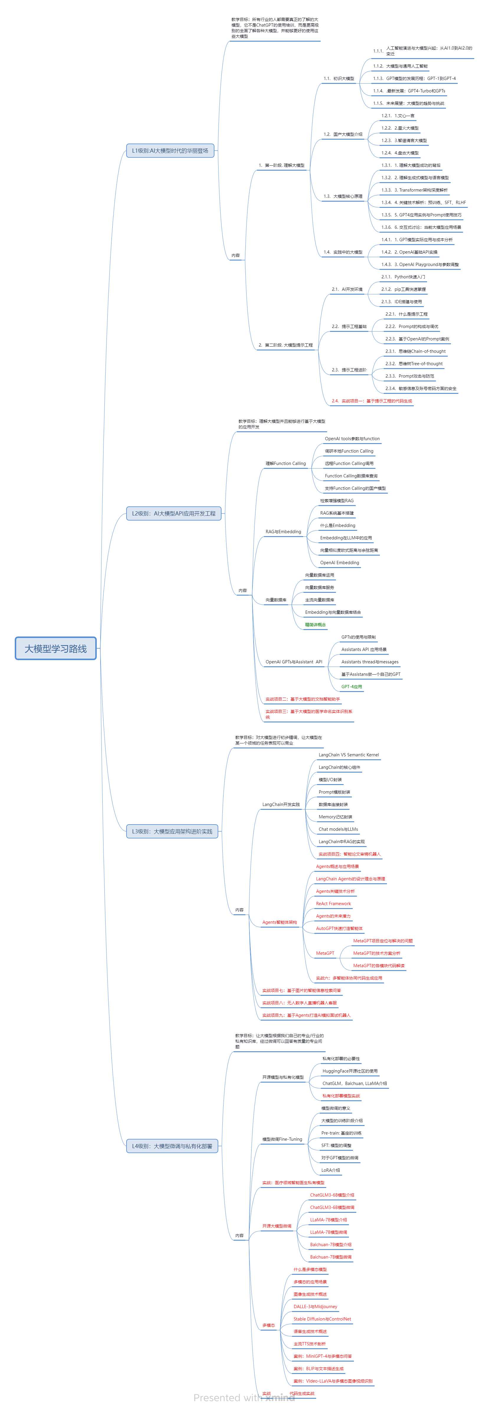
一、AGI大模型系统学习路线

很多人学习大模型的时候没有方向，东学一点西学一点，像只无头苍蝇乱撞，我下面分享的这个学习路线希望能够帮助到你们学习AI大模型。

二、AI大模型视频教程

三、AI大模型各大学习书籍

四、AI大模型各大场景实战案例

五、结束语

学习AI大模型是当前科技发展的趋势，它不仅能够为我们提供更多的机会和挑战，还能够让我们更好地理解和应用人工智能技术。通过学习AI大模型，我们可以深入了解深度学习、神经网络等核心概念，并将其应用于自然语言处理、计算机视觉、语音识别等领域。同时，掌握AI大模型还能够为我们的职业发展增添竞争力，成为未来技术领域的领导者。

再者，学习AI大模型也能为我们自己创造更多的价值，提供更多的岗位以及副业创收，让自己的生活更上一层楼。

因此，学习AI大模型是一项有前景且值得投入的时间和精力的重要选择。