


目录
一、基础知识
1.1 为什么选择序列模型?
序列模型能够应用在许多领域,例如:
-
语音识别
-
音乐发生器
-
情感分类
-
DNA序列分析
-
机器翻译
-
视频动作识别
-
命名实体识别

这些序列模型基本都属于监督式学习,输入x和输出y不一定都是序列模型。如果都是序列模型的话,模型长度不一定完全一致。
1.2 数学符号
下面以命名实体识别为例,介绍序列模型的命名规则。示例语句为:
Harry Potter and Hermione Granger invented a new spell.
该句话包含9个单词,输出y即为1 x 9向量,每位表征对应单词是否为人名的一部分,1表示是,0表示否。很明显,该句话中“Harry”,“Potter”,“Hermione”,“Granger”均是人名成分,所以,对应的输出y可表示为:
y=[1 1 0 1 1 0 0 0 0]
一般约定使用 ![]() 表示序列对应位置的输出,使用
表示序列对应位置的输出,使用 ![]() 表示输出序列长度,则1≤t≤Ty。
表示输出序列长度,则1≤t≤Ty。
对于输入x,表示为:
![]()
同样,![]() 表示序列对应位置的输入,
表示序列对应位置的输入,![]() 表示输入序列长度。注意,此例中,
表示输入序列长度。注意,此例中,![]() ,但是也存在
,但是也存在 ![]() 的情况
的情况
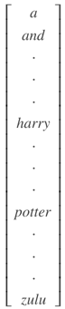
如何来表示每个![]() 呢?方法是首先建立一个词汇库vocabulary,尽可能包含更多的词汇。例如一个包含10000个词汇的词汇库为:
呢?方法是首先建立一个词汇库vocabulary,尽可能包含更多的词汇。例如一个包含10000个词汇的词汇库为:
然后,使用one-hot编码,例句中的每个单词 ![]() 都可以表示成10000 x 1的向量,词汇表中与
都可以表示成10000 x 1的向量,词汇表中与 ![]() 对应的位置为1,其它位置为0。该
对应的位置为1,其它位置为0。该 ![]() 为one-hot向量。值得一提的是如果出现词汇表之外的单词,可以使用UNK或其他字符串来表示。
为one-hot向量。值得一提的是如果出现词汇表之外的单词,可以使用UNK或其他字符串来表示。
对于多样本,以上序列模型对应的命名规则可表示为:![]() 。其中,i表示第i个样本。不同样本的
。其中,i表示第i个样本。不同样本的![]() 都有可能不同。
都有可能不同。
1.3 循环神经网络
对于序列模型,如果使用标准的神经网络,其模型结构如下:
使用标准的神经网络模型存在两个问题:
第一个问题,不同样本的输入序列长度或输出序列长度不同,即 ![]() ,造成模型难以统一。解决办法之一是设定一个最大序列长度,对每个输入和输出序列补零并统一到最大长度。但是这种做法实际效果并不理想。
,造成模型难以统一。解决办法之一是设定一个最大序列长度,对每个输入和输出序列补零并统一到最大长度。但是这种做法实际效果并不理想。
第二个问题,也是主要问题,这种标准神经网络结构无法共享序列不同 ![]() 之间的特征。例如,如果某个
之间的特征。例如,如果某个 ![]() 即“Harry”是人名成分,那么句子其它位置出现了“Harry”,也很可能也是人名。这是共享特征的结果,如同CNN网络特点一样。但是,上图所示的网络不具备共享特征的能力。值得一提的是,共享特征还有助于减少神经网络中的参数数量,一定程度上减小了模型的计算复杂度。例如上图所示的标准神经网络,假设每个
即“Harry”是人名成分,那么句子其它位置出现了“Harry”,也很可能也是人名。这是共享特征的结果,如同CNN网络特点一样。但是,上图所示的网络不具备共享特征的能力。值得一提的是,共享特征还有助于减少神经网络中的参数数量,一定程度上减小了模型的计算复杂度。例如上图所示的标准神经网络,假设每个 ![]() 扩展到最大序列长度为100,且词汇表长度为10000,则输入层就已经包含了100 x 10000个神经元了,权重参数很多,运算量将是庞大的。
扩展到最大序列长度为100,且词汇表长度为10000,则输入层就已经包含了100 x 10000个神经元了,权重参数很多,运算量将是庞大的。
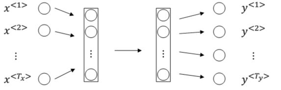
标准的神经网络不适合解决序列模型问题,而循环神经网络(RNN)是专门用来解决序列模型问题的。RNN模型结构如下:

序列模型从左到右,依次传递,此例中,![]() 之间是隐藏神经元。
之间是隐藏神经元。![]() 会传入到第 t+1 个元素中,作为输入。其中,a<0> 一般为零向量。
会传入到第 t+1 个元素中,作为输入。其中,a<0> 一般为零向量。
RNN模型包含三类权重系数,分别是![]() 且不同元素之间同一位置共享同一权重系数。
且不同元素之间同一位置共享同一权重系数。

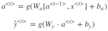
RNN的正向传播(Forward Propagation)过程为:
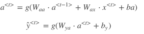
其中,g(⋅) 表示激活函数,不同的问题需要使用不同的激活函数。
为了简化表达式,可以对 ![]() 项进行整合:
项进行整合:
![]()
则正向传播可表示为:
值得一提的是,以上所述的RNN为单向RNN,即按照从左到右顺序,单向进行,![]() 只与左边的元素有关。但是,有时候
只与左边的元素有关。但是,有时候![]() 也可能与右边元素有关。例如下面两个句子中,单凭前三个单词,无法确定“Teddy”是否为人名,必须根据右边单词进行判断。
也可能与右边元素有关。例如下面两个句子中,单凭前三个单词,无法确定“Teddy”是否为人名,必须根据右边单词进行判断。
He said, “Teddy Roosevelt was a great President.”
He said, “Teddy bears are on sale!”
因此,有另外一种RNN结构是双向RNN,简称为BRNN。![]() 与左右元素均有关系,我们之后再详细介绍。
与左右元素均有关系,我们之后再详细介绍。
1.4 循环神经网络的反向传播
针对上面识别人名的例子,经过RNN正向传播,单个元素的Loss function为:
![]()
该样本所有元素的Loss function为:
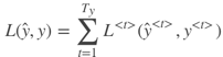
然后,反向传播(Backpropagation)过程就是从右到左分别计算L(ŷ ,y) 对参数 ![]() 的偏导数。思路与做法与标准的神经网络是一样的。一般可以通过成熟的深度学习框架自动求导,例如PyTorch、Tensorflow等。这种从右到左的求导过程被称为Backpropagation through time。
的偏导数。思路与做法与标准的神经网络是一样的。一般可以通过成熟的深度学习框架自动求导,例如PyTorch、Tensorflow等。这种从右到左的求导过程被称为Backpropagation through time。
1.5 不同类型的循环神经网络
以上介绍的例子中,Tx=Ty 。但是在很多RNN模型中,Tx 是不等于Ty 的。例如第1节介绍的许多模型都是Tx≠Ty。根据Tx与Ty的关系,RNN模型包含以下几个类型:

不同类型相应的示例结构如下:

1.6 语言模型和序列生成
语言模型是自然语言处理(NLP)中最基本和最重要的任务之一。使用RNN能够很好地建立需要的不同语言风格的语言模型。
什么是语言模型呢?举个例子,在语音识别中,某句语音有两种翻译:
-
The apple and pair salad.
-
The apple and pear salad.
很明显,第二句话更有可能是正确的翻译。语言模型实际上会计算出这两句话各自的出现概率。比如第一句话概率为![]() ,第二句话概率为
,第二句话概率为 ![]() 。也就是说,利用语言模型得到各自语句的概率,选择概率最大的语句作为正确的翻译。概率计算的表达式为:
。也就是说,利用语言模型得到各自语句的概率,选择概率最大的语句作为正确的翻译。概率计算的表达式为:
![]()
如何使用RNN构建语言模型?首先,我们需要一个足够大的训练集,训练集由大量的单词语句语料库(corpus)构成。然后,对corpus的每句话进行切分词(tokenize)。做法就跟第2节介绍的一样,建立vocabulary,对每个单词进行one-hot编码。例如下面这句话:
The Egyptian Mau is a bread of cat.
One-hot编码已经介绍过了,不再赘述。还需注意的是,每句话结束末尾,需要加上< EOS >作为语句结束符。另外,若语句中有词汇表中没有的单词,用< UNK >表示。假设单词“Mau”不在词汇表中,则上面这句话可表示为:
The Egyptian < UNK > is a bread of cat. < EOS >
准备好训练集并对语料库进行切分词等处理之后,接下来构建相应的RNN模型。

语言模型的RNN结构如上图所示,![]() 均为零向量。Softmax输出层
均为零向量。Softmax输出层 ![]() 表示出现该语句第一个单词的概率,softmax输出层
表示出现该语句第一个单词的概率,softmax输出层 ![]() 表示在第一个单词基础上出现第二个单词的概率,即条件概率,以此类推,最后是出现< EOS >的条件概率。
表示在第一个单词基础上出现第二个单词的概率,即条件概率,以此类推,最后是出现< EOS >的条件概率。
单个元素的softmax loss function为:
![]()
该样本所有元素的Loss function为:
![]()
对语料库的每条语句进行RNN模型训练,最终得到的模型可以根据给出语句的前几个单词预测其余部分,将语句补充完整。例如给出“Cats average 15”,RNN模型可能预测完整的语句是“Cats average 15 hours of sleep a day.”。
最后补充一点,整个语句出现的概率等于语句中所有元素出现的条件概率乘积。例如某个语句包含![]() 则整个语句出现的概率为:
则整个语句出现的概率为:
![]()
1.7 对新序列采样
在你训练一个序列模型之后,要想了解到这个模型学到了什么,一种非正式的方法就是进行一次新序列采样。
利用训练好的RNN语言模型,可以进行新的序列采样,从而随机产生新的语句。与上一节介绍的一样,相应的RNN模型如下所示:

首先,从第一个元素输出![]() 的softmax分布中随机选取一个word作为新语句的首单词。然后,
的softmax分布中随机选取一个word作为新语句的首单词。然后,![]() 作为
作为![]() ,得到
,得到![]() 的softmax分布。从中选取概率最大的word作为
的softmax分布。从中选取概率最大的word作为![]() ,继续将
,继续将![]() 作为
作为![]() ,以此类推。直到产生< EOS >结束符,则标志语句生成完毕。当然,也可以设定语句长度上限,达到长度上限即停止生成新的单词。最终,根据随机选择的首单词,RNN模型会生成一条新的语句。
,以此类推。直到产生< EOS >结束符,则标志语句生成完毕。当然,也可以设定语句长度上限,达到长度上限即停止生成新的单词。最终,根据随机选择的首单词,RNN模型会生成一条新的语句。
值得一提的是,如果不希望新的语句中包含< UNK >标志符,可以在每次产生< UNK >时重新采样,直到生成非< UNK >标志符为止。
以上介绍的是word level RNN,即每次生成单个word,语句由多个words构成。另外一种情况是character level RNN,即词汇表由单个英文字母或字符组成,如下所示:
![]()
Character level RNN与word level RNN不同的是,![]() 由单个字符组成而不是word。训练集中的每句话都当成是由许多字符组成的。character level RNN的优点是能有效避免遇到词汇表中不存在的单词< UNK >。但是,character level RNN的缺点也很突出。由于是字符表征,每句话的字符数量很大,这种大的跨度不利于寻找语句前部分和后部分之间的依赖性。另外,character level RNN的在训练时的计算量也是庞大的。基于这些缺点,目前character level RNN的应用并不广泛,但是在特定应用下仍然有发展的趋势。
由单个字符组成而不是word。训练集中的每句话都当成是由许多字符组成的。character level RNN的优点是能有效避免遇到词汇表中不存在的单词< UNK >。但是,character level RNN的缺点也很突出。由于是字符表征,每句话的字符数量很大,这种大的跨度不利于寻找语句前部分和后部分之间的依赖性。另外,character level RNN的在训练时的计算量也是庞大的。基于这些缺点,目前character level RNN的应用并不广泛,但是在特定应用下仍然有发展的趋势。
1.8 循环神经网络的梯度消失
基本的RNN算法还有一个很大的问题,就是梯度消失的问题。
如:语句中可能存在跨度很大的依赖关系,即某个word可能与它距离较远的某个word具有强依赖关系。例如下面这两条语句:
The cat, which already ate fish, was full.
The cats, which already ate fish, were full.
第一句话中,was受cat影响;第二句话中,were受cats影响。它们之间都跨越了很多单词。而一般的RNN模型每个元素受其周围附近的影响较大,难以建立跨度较大的依赖性。上面两句话的这种依赖关系,由于跨度很大,普通的RNN网络容易出现梯度消失,捕捉不到它们之间的依赖,造成语法错误。
解释原因:

之前讨论的训练很深的网络,我们讨论了梯度消失的问题。比如说一个很深很深的网络(上图编号4所示),100层,甚至更深,对这个网络从左到右做前向传播然后再反向传播。我们知道如果这是个很深的神经网络,从输出y得到的梯度很难传播回去,很难影响靠前层的权重,很难影响前面层(编号5所示的层)的计算。
对于有同样问题的RNN,首先从左到右前向传播,然后反向传播。但是反向传播会很困难,因为同样的梯度消失的问题,后面层的输出误差(上图编号6所示)很难影响前面层(上图编号7所示的层)的计算。这就意味着,实际上很难让一个神经网络能够意识到它要记住看到的是单数名词还是复数名词,然后在序列后面生成依赖单复数形式的was或者were。
另一方面,RNN也可能出现梯度爆炸的问题,即gradient过大。常用的解决办法是设定一个阈值,一旦梯度最大值达到这个阈值,就对整个梯度向量进行尺度缩小。这种做法被称为gradient clipping。
1.9 GRU单元(门控循环单元)
门控循环单元,它改变了RNN的隐藏层,使其可以更好地捕捉深层连接,并改善了梯度消失问题。更好捕捉非常长范围的依赖,让RNN更加有效。
RNN的隐藏层单元结构如下图所示:

![]() 的表达式为:
的表达式为: ![]()
为了解决梯度消失问题,对上述单元进行修改,添加了记忆单元,构建GRU,如下图所示:

相应的表达式为:
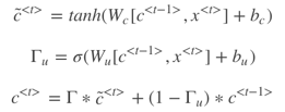
其中,![]() ,
, ![]() 意为gate,记忆单元。1Γu=1时,代表更新;当Γu=0 时,代表记忆,保留之前的模块输出。这一点跟CNN中的ResNets的作用有点类似。因此,Γu能够保证RNN模型中跨度很大的依赖关系不受影响,消除梯度消失问题。
意为gate,记忆单元。1Γu=1时,代表更新;当Γu=0 时,代表记忆,保留之前的模块输出。这一点跟CNN中的ResNets的作用有点类似。因此,Γu能够保证RNN模型中跨度很大的依赖关系不受影响,消除梯度消失问题。
上面介绍的是简化的GRU模型,完整的GRU添加了另外一个gate,即ΓrΓr,表达式如下:
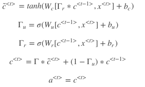
注意,以上表达式中的∗∗表示元素相乘,而非矩阵相乘。
1.10 长短期记忆
上面你已经学了GRU(门控循环单元)。它能够让你可以在序列中学习非常深的连接。其他类型的单元也可以让你做到这个,比如LSTM即长短时记忆网络,甚至比GRU更加有效,让我们看看。
LSTM是另一种更强大的解决梯度消失问题的方法。它对应的RNN隐藏层单元结构如下图所示:

相应的表达式为:
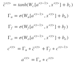
LSTM包含三个gates:Γu,Γf,Γo,分别对应update gate,forget gate和output gate。
如果考虑![]() 对Γu,Γf,Γo的影响,可加入peephole connection,对LSTM的表达式进行修改
对Γu,Γf,Γo的影响,可加入peephole connection,对LSTM的表达式进行修改

GRU可以看成是简化的LSTM,两种方法都具有各自的优势。
1.11 双向循环神经网络
它的结构如下图所示:

BRNN对应的输出 ![]() 表达式为 :
表达式为 : ![]()
BRNN能够同时对序列进行双向处理,性能大大提高。但是计算量较大,且在处理实时语音时,需要等到完整的一句话结束时才能进行分析。
1.12 深层循环神经网络
Deep RNNs由多层RNN组成,其结构如下图所示:

与DNN一样,用上标 [l] 表示层数。Deep RNNs中 ![]() 的表达式为:
的表达式为:
![]()
我们知道DNN层数可达100多,而Deep RNNs一般没有那么多层,3层RNNs已经较复杂了。
另外一种Deep RNNs结构是每个输出层上还有一些垂直单元,如下图所示:

二、测验
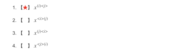
1、假设你的训练样本是句子(单词序列),下面哪个选项指的是第i个训练样本中的第j个词?
2、看一下下面的这个循环神经网络:

在下面的条件中,满足上图中的网络结构的参数是:
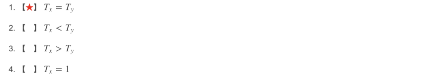
上图中每一个输入都与输出相匹配。
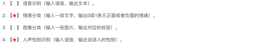
3、这些任务中的哪一个会使用多对一的RNN体系结构?

4、假设你现在正在训练下面这个RNN的语言模型:

在t时,这个RNN在做什么?
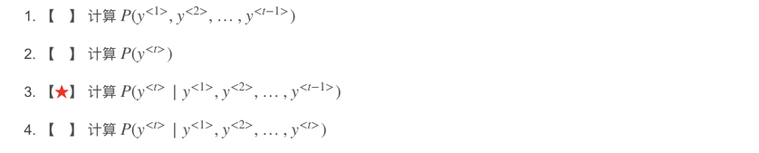
是的,这个语言模型正在试着根据前面所有的知识来预测下一步。
5、你已经完成了一个语言模型RNN的训练,并用它来对句子进行随机取样,如下图:

在每个时间步tt都在做什么?

6、你正在训练一个RNN网络,你发现你的权重与激活值都是“NaN”,下列选项中,哪一个是导致这个问题的最有可能的原因?

7、假设你正在训练一个LSTM网络,你有一个10,000词的词汇表,并且使用一个激活值维度为100的LSTM块,在每一个时间步中,Γu的维度是多少?
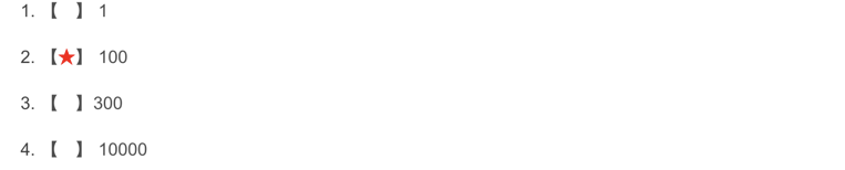
Γu的向量维度等于LSTM中隐藏单元的数量。
8、这里有一些GRU的更新方程:


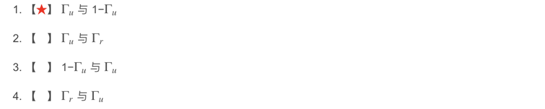
9、这里有一些GRU和LSTM的方程:

从这些我们可以看到,在LSTM中的更新门和遗忘门在GRU中扮演类似 ⎯⎯⎯⎯⎯⎯⎯⎯⎯_与⎯⎯⎯⎯⎯⎯⎯⎯⎯_的角色,空白处应该填什么?
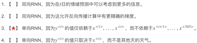
10、你有一只宠物狗,它的心情很大程度上取决于当前和过去几天的天气。你已经收集了过去365天的天气数据![]() ,这些数据是一个序列,你还收集了你的狗心情的数据
,这些数据是一个序列,你还收集了你的狗心情的数据 ![]() ,你想建立一个模型来从x到y进行映射,你应该使用单向RNN还是双向RNN来解决这个问题?
,你想建立一个模型来从x到y进行映射,你应该使用单向RNN还是双向RNN来解决这个问题?
三、编程
3.1 一步步创建循环神经网络
下面的编程作业中,将用 numpy 实现第一个循环神经网络。
循环神经网络(RNN)对自然语言处理和其他序列任务非常有效,因为它们具有“memory”。 他们可以读取输入内容 ![]() (例如一个单词)并通过隐藏层激活函数记住一些 信息或上下文 并从一个时间步传递到下一个时间步。单向RNN 处理后的信息作为下一个的输入。双向RNN 序列模型是从左往右传递然后再从右往左传递。
(例如一个单词)并通过隐藏层激活函数记住一些 信息或上下文 并从一个时间步传递到下一个时间步。单向RNN 处理后的信息作为下一个的输入。双向RNN 序列模型是从左往右传递然后再从右往左传递。
3.1.1 基本循环神经网络的正向传播
import numpy as np
# 自定义工具包
from rnn_utils import *
之后,您将使用RNN生成音乐。 实现的基本RNN具有以下结构。 在这个例子中 𝑇𝑥=𝑇𝑦

实现RNN的方法:
Steps::
实施 RNN 的一个时间步所需的计算。
为了一次处理所有输入 实现循时间步长。
3.1.2 RNN 单元
循环神经网络可以看作是单个Cell 的重复。 您首先要在单个时间步上实现计算。 下图描述了RNN单元的单个时间步的操作。

说明:
1、使用tanh激活计算隐藏状态: ![]() 。
。
2、使用计算出来的隐藏状态 ![]() 去计算预测
去计算预测 ![]() ,借助 softmax 函数实现。
,借助 softmax 函数实现。
3、在缓存中存储 ![]() 。
。
4、返回 ![]() 和 缓存内容。
和 缓存内容。
下面我们矢量化 m 个样本 因此 ![]() 将有维度
将有维度 ![]() ,
,![]() 将有维度
将有维度 ![]()
import numpy as np


def softmax(x):
    e_x = np.exp(x - np.max(x))
    return e_x / e_x.sum(axis=0)


def rnn_cell_forward(xt, a_prev, parameters):
    """
    实现 RNN-cell 的单个正向步骤,如图(2)所述

    参数:
    xt -- your input data at timestep "t", numpy array of shape (n_x, m).
    a_prev -- Hidden state at timestep "t-1", numpy array of shape (n_a, m)
    parameters -- python dictionary containing:
                        Wax -- Weight matrix multiplying the input, numpy array of shape (n_a, n_x)
                        Waa -- Weight matrix multiplying the hidden state, numpy array of shape (n_a, n_a)
                        Wya -- Weight matrix relating the hidden-state to the output, numpy array of shape (n_y, n_a)
                        ba --  Bias, numpy array of shape (n_a, 1)
                        by -- Bias relating the hidden-state to the output, numpy array of shape (n_y, 1)
    Returns:
    a_next -- next hidden state, of shape (n_a, m)
    yt_pred -- prediction at timestep "t", numpy array of shape (n_y, m)
    cache -- tuple of values needed for the backward pass, contains (a_next, a_prev, xt, parameters)
    """

    # "parameters" 字典中检索需要的参数
    Wax = parameters["Wax"]
    Waa = parameters["Waa"]
    Wya = parameters["Wya"]
    ba = parameters["ba"]
    by = parameters["by"]

    # 使用上面给出的公式计算下一个激活状态
    a_next = np.tanh(np.dot(Waa, a_prev) + np.dot(Wax, xt) + ba)
    # 使用上面给出的公式计算当前单元的输出
    yt_pred = softmax(np.dot(Wya, a_next) + by)

    # 将需要向后传播的值存储在缓存中
    cache = (a_next, a_prev, xt, parameters)

    return a_next, yt_pred, cache


if __name__ == '__main__':
    np.random.seed(1)
    xt = np.random.randn(3, 10) # 生成 3 x 10 维度的数组
    a_prev = np.random.randn(5, 10)
    Waa = np.random.randn(5, 5)
    Wax = np.random.randn(5, 3)
    Wya = np.random.randn(2, 5)
    ba = np.random.randn(5, 1)
    by = np.random.randn(2, 1)
    parameters = {"Waa": Waa, "Wax": Wax, "Wya": Wya, "ba": ba, "by": by}

    a_next, yt_pred, cache = rnn_cell_forward(xt, a_prev, parameters)
    print("a_next[4] = ", a_next[4])
    print("a_next.shape = ", a_next.shape)
    print("yt_pred[1] =", yt_pred[1])
    print("yt_pred.shape = ", yt_pred.shape)
a_next[4] = [ 0.59584544 0.18141802 0.61311866 0.99808218 0.85016201 0.99980978
-0.18887155 0.99815551 0.6531151 0.82872037]
a_next.shape = (5, 10)
yt_pred[1] = [0.9888161 0.01682021 0.21140899 0.36817467 0.98988387 0.88945212
0.36920224 0.9966312 0.9982559 0.17746526]
yt_pred.shape = (2, 10)
结果分析:
xt生成结果显示:
a_prev生成结果显示:
Waa生成结果显示:
Wax生成结果显示:
Wya生成结果显示:

ba生成结果显示:
by生成结果显示:

a_next结果显示: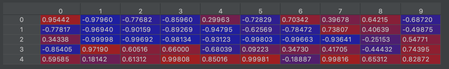
yt_pred结果显示:
3.1.3 RNN正向传播
您可以将RNN视为刚刚构建的 cell 的重复。 如果您输入的数据序列经过10个时间步长,则将复制RNN单元10次。 每个 Cell 都将前一个单元格 ![]() 的隐藏状态和当前时间步的输入数据
的隐藏状态和当前时间步的输入数据![]() 作为输入。 它为此时间步长输出隐藏状态
作为输入。 它为此时间步长输出隐藏状态![]() )和预测
)和预测![]() 。
。

说明:
1、创建 zeros (𝑎) 它将存储RNN计算出的所有隐藏状态。
2、初始化 “next”隐藏状态为 𝑎0
3、开始遍历每个时间步 ,您的增量索引为 𝑡 :
- 通过运行 rnn_step_forward 更新 “next”隐藏状态和cache
- 存储“next”隐藏状态在 a中
- 存储预测在 y中
- 添加 cache 到 caches中
4、返回 𝑎, 𝑦 和 caches
import numpy as np
def softmax(x):
e_x = np.exp(x - np.max(x))
return e_x / e_x.sum(axis=0)
def rnn_cell_forward(xt, a_prev, parameters):
"""
实现 RNN-cell 的单个正向步骤,如图(2)所述
参数:
xt -- your input data at timestep "t", numpy array of shape (n_x, m).
a_prev -- Hidden state at timestep "t-1", numpy array of shape (n_a, m)
parameters -- python dictionary containing:
Wax -- Weight matrix multiplying the input, numpy array of shape (n_a, n_x)
Waa -- Weight matrix multiplying the hidden state, numpy array of shape (n_a, n_a)
Wya -- Weight matrix relating the hidden-state to the output, numpy array of shape (n_y, n_a)
ba -- Bias, numpy array of shape (n_a, 1)
by -- Bias relating the hidden-state to the output, numpy array of shape (n_y, 1)
Returns:
a_next -- next hidden state, of shape (n_a, m)
yt_pred -- prediction at timestep "t", numpy array of shape (n_y, m)
cache -- tuple of values needed for the backward pass, contains (a_next, a_prev, xt, parameters)
"""
# "parameters" 字典中检索需要的参数
Wax = parameters["Wax"]
Waa = parameters["Waa"]
Wya = parameters["Wya"]
ba = parameters["ba"]
by = parameters["by"]
# 使用上面给出的公式计算下一个激活状态
a_next = np.tanh(np.dot(Waa, a_prev) + np.dot(Wax, xt) + ba) # 5 x 10
# 使用上面给出的公式计算当前单元的输出
yt_pred = softmax(np.dot(Wya, a_next) + by)
# 将需要向后传播的值存储在缓存中
cache = (a_next, a_prev, xt, parameters)
return a_next, yt_pred, cache
def rnn_forward(x, a0, parameters):
"""
实现RNN神经网络的正向传播
Arguments:
x -- Input data for every time-step, of shape (n_x, m, T_x).
a0 -- Initial hidden state, of shape (n_a, m)
parameters -- python dictionary containing:
Waa -- Weight matrix multiplying the hidden state, numpy array of shape (n_a, n_a)
Wax -- Weight matrix multiplying the input, numpy array of shape (n_a, n_x)
Wya -- Weight matrix relating the hidden-state to the output, numpy array of shape (n_y, n_a)
ba -- Bias numpy array of shape (n_a, 1)
by -- Bias relating the hidden-state to the output, numpy array of shape (n_y, 1)
Returns:
a -- Hidden states for every time-step, numpy array of shape (n_a, m, T_x)
y_pred -- Predictions for every time-step, numpy array of shape (n_y, m, T_x)
caches -- tuple of values needed for the backward pass, contains (list of caches, x)
"""
# 初始化“缓存”,其中将包含所有缓存的列表
caches = []
# 从 x 和 Wy 获取 shape
n_x, m, T_x = x.shape # n_x: 是输入 x 的维度 m:样本的数目 ;T_x 是序列的长度 4
n_y, n_a = parameters["Wya"].shape # n_y 的维度 2 ;n_a维度 5
# 用0初始化 "a" 和 "y"
a = np.zeros([n_a, m, T_x]) # 5 维度; 10个样本 ;序列长度 4
y_pred = np.zeros([n_y, m, T_x]) # 2 维 ;10个样本;序列长度 4
# 初始化 a_next
a_next = a0 # 5 x 10
# 循环遍历所有的 time-steps
for t in range(T_x):
# 更新下一个隐藏状态,计算预测,获取缓存
a_next, yt_pred, cache = rnn_cell_forward(x[:, :, t], a_next, parameters)
# 保存 "next" 隐藏状态值到 a (≈1 line)
a[:, :, t] = a_next
# 保存预测值到 y
y_pred[:, :, t] = yt_pred
# 添加 "cache" 到 "caches"
caches.append(cache)
# 存储后向传播需要的值到 cache
caches = (caches, x)
return a, y_pred, caches
if __name__ == '__main__':
np.random.seed(1)
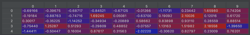
x = np.random.randn(3, 10, 4) # 输入的每个 Cell的 x 是3维的;10个样本 单元格数目(x 序列长度)是 4
a0 = np.random.randn(5, 10) # 每个样本的 a0 为 5x1 维的 ;这里的10 是指 10个样本的 a0情况, 每个样本的 a0 值不一样。
Waa = np.random.randn(5, 5) # 每个 Cell的 Waa权重都是 Waa 5 x 5
Wax = np.random.randn(5, 3) # 每个 Cell的 Wax权重都是 5 x 3
Wya = np.random.randn(2, 5) # 每个 Cell的 Wya权重都是 2x5
ba = np.random.randn(5, 1) # ba 表示每个 Cell的偏置都是 5 x 1
by = np.random.randn(2, 1) # y的每个Cell的输出都是2维的 p (1-p)
parameters = {"Waa": Waa, "Wax": Wax, "Wya": Wya, "ba": ba, "by": by}
a, y_pred, caches = rnn_forward(x, a0, parameters)
print("a[4][1] = ", a[4][1]) # 输出第二个样本中 各个Cell中 a第5维的值
print("a.shape = ", a.shape) # 5 x 10 x 4
print("y_pred[1][3] =", y_pred[1][3]) # 输出第4个样本中,各个Cell中 y是第1维的值
print("y_pred.shape = ", y_pred.shape)# (2, 10, 4)
print("caches[1][1][3] =", caches[1][1][3]) # 输出结果是 第四个样本中 每个Cell中 输入 x的第2维的值
print("len(caches) = ", len(caches))
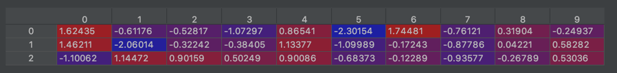
x的可视化结果:
a[4][1] = [-0.99999375 0.77911235 -0.99861469 -0.99833267]
a.shape = (5, 10, 4)
y_pred[1][3] = [0.79560373 0.86224861 0.11118257 0.81515947]
y_pred.shape = (2, 10, 4)
caches[1][1][3] = [-1.1425182 -0.34934272 -0.20889423 0.58662319]
len(caches) = 2
恭喜你! 您已经从头开始成功构建了循环神经网络的正向传播。 这对于某些应用程序将足够好,但是会遇到梯度消失的问题。 因此,每个输出 ![]() 要使用“local”上下文进行估算(对于输入的
要使用“local”上下文进行估算(对于输入的![]() ,
,![]() 距离不要离t太远)。
距离不要离t太远)。
在下一部分中,将构建一个更复杂的LSTM模型,该模型更适合解决逐渐消失的梯度。 LSTM将能够更好地记住一条信息并将其保存许多 timesteps。
3.2 长短期记忆(LSTM)网络
下图显示了LSTM单元的操作。

关于 gates:
- Forget gate
为了便于说明,假设我们正在阅读一段文本中的单词,并希望使用LSTM来跟踪语法结构,例如主题是单数还是复数。 如果主题从单数变为复数,我们需要找到一种方法来摆脱以前存储的单/复数状态的存储值。 在LSTM中,forget gate 使我们可以这样做:
![]()
在这里 𝑊𝑓是控制 Forget gate 行为的权重,上面的方程式得出向量 ![]() 的值介于 0~1之间,该 Forget gate 向量将逐元素乘以先前的单元状态
的值介于 0~1之间,该 Forget gate 向量将逐元素乘以先前的单元状态 ![]() 所以,
所以,![]() 的其中有值为0(或接近0),则表示LSTM应该删除
的其中有值为0(或接近0),则表示LSTM应该删除![]() 中相应组件的信息,如果
中相应组件的信息,如果![]() 值之一为1,则它将保留信息。
值之一为1,则它将保留信息。
- Update gate
一旦我们忘记了所讨论的主题是单数,就需要找到一种更新它的方法,以反映新主题现在是复数。 这是Update gate 的公式:
![]()
和 forget gate 相似,这里的![]() 的值 也是介于 0~1,这将和
的值 也是介于 0~1,这将和![]() 相乘 为了去计算
相乘 为了去计算 ![]()
- Updating the cell
要更新新主题,我们需要创建一个新的数字向量,可以将其添加到先前的单元格状态中。 我们使用的等式是:
![]()
最后,新的单元状态为:
![]()
- Output gate
为了确定我们将使用哪些输出,我们将使用以下两个公式:
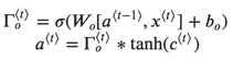
在方程式中,您决定使用 sigmoid 函数输出;然后您将其乘以以前的状态 的tanh。
3.2.1 LSTM cell

练习:实现图中描述的LSTM单元。
说明:
1、在单个矩阵中串联 ![]()
![]()
2、计算所有公式2-6。 您可以使用sigmoid()(提供)和np.tanh()。
3、您可以使用softmax()(提供)计算预测 ![]() 。
。
import numpy as np

def softmax(x):
    e_x = np.exp(x - np.max(x))
    return e_x / e_x.sum(axis=0)

def sigmoid(x):
    return 1 / (1 + np.exp(-x))

def lstm_cell_forward(xt, a_prev, c_prev, parameters):
    """
    实现图4中 LSTM Cell的单个正向步骤

    参数:
    xt -- your input data at timestep "t", numpy array of shape (n_x, m).
    a_prev -- Hidden state at timestep "t-1", numpy array of shape (n_a, m)
    c_prev -- Memory state at timestep "t-1", numpy array of shape (n_a, m)
    parameters -- python dictionary containing:
                        Wf -- Weight matrix of the forget gate, numpy array of shape (n_a, n_a + n_x)
                        bf -- Bias of the forget gate, numpy array of shape (n_a, 1)
                        Wi -- Weight matrix of the save gate, numpy array of shape (n_a, n_a + n_x)
                        bi -- Bias of the save gate, numpy array of shape (n_a, 1)
                        Wc -- Weight matrix of the first "tanh", numpy array of shape (n_a, n_a + n_x)
                        bc --  Bias of the first "tanh", numpy array of shape (n_a, 1)
                        Wo -- Weight matrix of the focus gate, numpy array of shape (n_a, n_a + n_x)
                        bo --  Bias of the focus gate, numpy array of shape (n_a, 1)
                        Wy -- Weight matrix relating the hidden-state to the output, numpy array of shape (n_y, n_a)
                        by -- Bias relating the hidden-state to the output, numpy array of shape (n_y, 1)

    Returns:
    a_next -- next hidden state, of shape (n_a, m)
    c_next -- next memory state, of shape (n_a, m)
    yt_pred -- prediction at timestep "t", numpy array of shape (n_y, m)
    cache -- tuple of values needed for the backward pass, contains (a_next, c_next, a_prev, c_prev, xt, parameters)

    Note: ft/it/ot stand for the forget/update/output gates, cct stands for the candidate value (c tilda),
          c stands for the memory value
    """

    # 从 "parameters" 字典中检索参数
    Wf = parameters["Wf"]
    bf = parameters["bf"]
    Wi = parameters["Wi"]
    bi = parameters["bi"]
    Wc = parameters["Wc"]
    bc = parameters["bc"]
    Wo = parameters["Wo"]
    bo = parameters["bo"]
    Wy = parameters["Wy"]
    by = parameters["by"]

    # 从xt和Wy shape中检索维度
    n_x, m = xt.shape  # n_x是3维;m是样本数
    n_y, n_a = Wy.shape  # (2 x 5)

    # 串联 a_prev 和 xt
    concat = np.zeros([n_a + n_x, m])  # 8 x 10维
    concat[: n_a, :] = a_prev
    concat[n_a:, :] = xt

    # 使用图4中给定的公式 计算ft,it,cct,c_next,ot,a_next的值
    ft = sigmoid(np.dot(Wf, concat) + bf)
    it = sigmoid(np.dot(Wi, concat) + bi)
    cct = np.tanh(np.dot(Wc, concat) + bc)
    c_next = ft * c_prev + it * cct
    ot = sigmoid(np.dot(Wo, concat) + bo)
    a_next = ot * np.tanh(c_next)

    # 计算LSTM单元的预测
    yt_pred = softmax(np.dot(Wy, a_next) + by)

    # 将向后传播所需的值存储在缓存中 cache
    cache = (a_next, c_next, a_prev, c_prev, ft, it, cct, ot, xt, parameters)

    return a_next, c_next, yt_pred, cache


if __name__ == '__main__':

    np.random.seed(1)
    xt = np.random.randn(3, 10)  # 10个样本,每个样本的输入 x 是3维的
    a_prev = np.random.randn(5, 10)  # 这里的10 是指 10个样本a_prev的情况 ;每个样本的a_prev是 5x1 维的,每个样本的a_prev值不同
    c_prev = np.random.randn(5, 10)  # 这里的10 是指 10个样本 c_prev 的情况 ;每个样本的 c_prev 是 5x1 维的,每个样本的 c_prev 值不同
    Wf = np.random.randn(5, 5 + 3)
    bf = np.random.randn(5, 1)
    Wi = np.random.randn(5, 5 + 3)
    bi = np.random.randn(5, 1)
    Wo = np.random.randn(5, 5 + 3)
    bo = np.random.randn(5, 1)
    Wc = np.random.randn(5, 5 + 3)
    bc = np.random.randn(5, 1)
    Wy = np.random.randn(2, 5)
    by = np.random.randn(2, 1)

    parameters = {"Wf": Wf, "Wi": Wi, "Wo": Wo, "Wc": Wc, "Wy": Wy, "bf": bf, "bi": bi, "bo": bo, "bc": bc, "by": by}

    a_next, c_next, yt, cache = lstm_cell_forward(xt, a_prev, c_prev, parameters)
    print("a_next[4] = ", a_next[4])
    print("a_next.shape = ", c_next.shape)
    print("c_next[2] = ", c_next[2])
    print("c_next.shape = ", c_next.shape)
    print("yt[1] =", yt[1])
    print("yt.shape = ", yt.shape)
    print("cache[1][3] =", cache[1][3])
    print("len(cache) = ", len(cache))
输出结果:
a_next[4] = [-0.66408471 0.0036921 0.02088357 0.22834167 -0.85575339 0.00138482
0.76566531 0.34631421 -0.00215674 0.43827275]
a_next.shape = (5, 10)
c_next[2] = [ 0.63267805 1.00570849 0.35504474 0.20690913 -1.64566718 0.11832942
0.76449811 -0.0981561 -0.74348425 -0.26810932]
c_next.shape = (5, 10)
yt[1] = [0.79913913 0.15986619 0.22412122 0.15606108 0.97057211 0.31146381
0.00943007 0.12666353 0.39380172 0.07828381]
yt.shape = (2, 10)
cache[1][3] = [-0.16263996 1.03729328 0.72938082 -0.54101719 0.02752074 -0.30821874
0.07651101 -1.03752894 1.41219977 -0.37647422]
len(cache) = 10
3.2.2 LSTM 正向传播
既然您已经实现了LSTM的一个步骤,现在就可以使用for循环对此序列进行迭代,以处理 ![]() 输入序列。
输入序列。

练习:实现lstm_forward()去运行 LSTM 的时间步长。
Note:![]() 初始化为0。
初始化为0。
def lstm_forward(x, a0, parameters):
    """
    使用上面描述的 LSTM-cell 实现循环神经网络的正向传播

    Arguments:
    x -- Input data for every time-step, of shape (n_x, m, T_x).
    a0 -- Initial hidden state, of shape (n_a, m)
    parameters -- python dictionary containing:
                        Wf -- Weight matrix of the forget gate, numpy array of shape (n_a, n_a + n_x)
                        bf -- Bias of the forget gate, numpy array of shape (n_a, 1)
                        Wi -- Weight matrix of the save gate, numpy array of shape (n_a, n_a + n_x)
                        bi -- Bias of the save gate, numpy array of shape (n_a, 1)
                        Wc -- Weight matrix of the first "tanh", numpy array of shape (n_a, n_a + n_x)
                        bc -- Bias of the first "tanh", numpy array of shape (n_a, 1)
                        Wo -- Weight matrix of the focus gate, numpy array of shape (n_a, n_a + n_x)
                        bo -- Bias of the focus gate, numpy array of shape (n_a, 1)
                        Wy -- Weight matrix relating the hidden-state to the output, numpy array of shape (n_y, n_a)
                        by -- Bias relating the hidden-state to the output, numpy array of shape (n_y, 1)

    Returns:
    a -- Hidden states for every time-step, numpy array of shape (n_a, m, T_x)
    y -- Predictions for every time-step, numpy array of shape (n_y, m, T_x)
    caches -- tuple of values needed for the backward pass, contains (list of all the caches, x)
    """

    # 初始化缓存列表
    caches = []

    # Retrieve dimensions from shapes of xt and Wy (≈2 lines)
    n_x, m, T_x = x.shape # (3 x 7)
    n_y, n_a = parameters['Wy'].shape # (2 x 5)

    # 初始化 "a", "c" 和 "y" 为0
    a = np.zeros([n_a, m, T_x])
    c = np.zeros([n_a, m, T_x])
    y = np.zeros([n_y, m, T_x])

    # 初始化 a_next 和 c_next
    a_next = a0
    c_next = np.zeros([n_a, m])

    # 循环遍历所有的 time-steps
    for t in range(T_x):
        # Update next hidden state, next memory state, compute the prediction, get the cache (≈1 line)
        a_next, c_next, yt, cache = lstm_cell_forward(x[:, :, t], a_next, c_next, parameters)
        # Save the value of the new "next" hidden state in a (≈1 line)
        a[:, :, t] = a_next
        # Save the value of the prediction in y (≈1 line)
        y[:, :, t] = yt
        # Save the value of the next cell state (≈1 line)
        c[:, :, t] = c_next
        # Append the cache into caches (≈1 line)
        caches.append(cache)


    caches = (caches, x)

    return a, y, c, caches


if __name__ == '__main__':

    np.random.seed(1)
    x = np.random.randn(3, 10, 7)  # 输入的每个 Cell的 x 是3维的;10个样本 单元格数目(x 序列长度)是 7
    a0 = np.random.randn(5, 10)  # 每个样本的 a0 为 5x1 维的 ;这里的10 是指 10个样本的 a0情况, 每个样本的 a0 值不一样。
    Wf = np.random.randn(5, 5 + 3)  # 每个 Cell的  Wf 权重都是 5 x 8
    bf = np.random.randn(5, 1)
    Wi = np.random.randn(5, 5 + 3)  # 每个 Cell的  Wi 权重都是 5 x 8
    bi = np.random.randn(5, 1)
    Wo = np.random.randn(5, 5 + 3)  # 每个 Cell的  Wo 权重都是 5 x 8
    bo = np.random.randn(5, 1)
    Wc = np.random.randn(5, 5 + 3)  # 每个 Cell的  Wc 权重都是 5 x 8
    bc = np.random.randn(5, 1)
    Wy = np.random.randn(2, 5)  # 每个 Cell的  Wy 权重都是 2 x 5
    by = np.random.randn(2, 1)

    parameters = {"Wf": Wf, "Wi": Wi, "Wo": Wo, "Wc": Wc, "Wy": Wy, "bf": bf, "bi": bi, "bo": bo, "bc": bc, "by": by}

    a, y, c, caches = lstm_forward(x, a0, parameters)
    print("a[4][3][6] = ", a[4][3][6])
    print("a.shape = ", a.shape)
    print("y[1][4][3] =", y[1][4][3])
    print("y.shape = ", y.shape)
    print("caches[1][1[1]] =", caches[1][1][1])
    print("c[1][2][1]", c[1][2][1])
    print("len(caches) = ", len(caches))
输出结果:
a[4][3][6] = 0.17211776753291672
a.shape = (5, 10, 7)
y[1][4][3] = 0.9508734618501101
y.shape = (2, 10, 7)
caches[1][1[1]] = [ 0.82797464 0.23009474 0.76201118 -0.22232814 -0.20075807 0.18656139
0.41005165]
c[1][2][1] -0.8555449167181982
len(caches) = 2
3.3 循环神经网络的反向传播(可选)
在现代深度学习框架中,您只需要实现前向传递,并且框架会处理后向传递,因此大多数深度学习工程师无需理会后向传递的细节。 但是,如果您是微积分专家并且想查看RNN中反向传播的详细信息,则可以遍历 NoteBook中的可选部分。
在较早的课程中,当您实现了一个简单的(完全连接的)神经网络时,您就使用了反向传播来计算关于更新参数的成本的导数。 同样,在循环神经网络中,您可以计算成本的导数以更新参数。 反向传播方程非常复杂,我们在视频中没有求解它们。 但是,我们将在下面简要介绍它们。
3.3.1 基本的RNN反向传播
我们从计算基本RNN单元的反向传播开始。

要计算rnn_cell_backward,您需要计算以下方程式。 手工导出它们是一个很好的练习。
def rnn_cell_backward(da_next, cache):
    """
    实现RNN-cell的反向传播

    Arguments:
    da_next -- Gradient of loss with respect to next hidden state
    cache -- python dictionary containing useful values (output of rnn_step_forward())

    Returns:
    gradients -- python dictionary containing:
                        dx -- Gradients of input data, of shape (n_x, m)
                        da_prev -- Gradients of previous hidden state, of shape (n_a, m)
                        dWax -- Gradients of input-to-hidden weights, of shape (n_a, n_x)
                        dWaa -- Gradients of hidden-to-hidden weights, of shape (n_a, n_a)
                        dba -- Gradients of bias vector, of shape (n_a, 1)
    """

    # 从缓存中检出值
    (a_next, a_prev, xt, parameters) = cache

    # 从parameters 参数字典中检出值
    Wax = parameters["Wax"]
    Waa = parameters["Waa"]
    Wya = parameters["Wya"]
    ba = parameters["ba"]
    by = parameters["by"]

    dtanh = (1 - a_next * a_next) * da_next

    dxt = np.dot(Wax.T, dtanh)
    dWax = np.dot(dtanh, xt.T)

    da_prev = np.dot(Waa.T, dtanh)
    dWaa = np.dot(dtanh, a_prev.T)

    dba = np.sum(dtanh, keepdims=True, axis=-1)

    gradients = {"dxt": dxt, "da_prev": da_prev, "dWax": dWax, "dWaa": dWaa, "dba": dba}

    return gradients


if __name__ == '__main__':

    np.random.seed(1)
    xt = np.random.randn(3, 10)
    a_prev = np.random.randn(5, 10)
    Wax = np.random.randn(5, 3)
    Waa = np.random.randn(5, 5)
    Wya = np.random.randn(2, 5)
    ba = np.random.randn(5, 1)
    by = np.random.randn(2, 1)
    parameters = {"Wax": Wax, "Waa": Waa, "Wya": Wya, "ba": ba, "by": by}

    a_next, yt, cache = rnn_cell_forward(xt, a_prev, parameters)

    da_next = np.random.randn(5, 10)
    gradients = rnn_cell_backward(da_next, cache)
    print("gradients[\"dxt\"][1][2] =", gradients["dxt"][1][2])
    print("gradients[\"dxt\"].shape =", gradients["dxt"].shape)
    print("gradients[\"da_prev\"][2][3] =", gradients["da_prev"][2][3])
    print("gradients[\"da_prev\"].shape =", gradients["da_prev"].shape)
    print("gradients[\"dWax\"][3][1] =", gradients["dWax"][3][1])
    print("gradients[\"dWax\"].shape =", gradients["dWax"].shape)
    print("gradients[\"dWaa\"][1][2] =", gradients["dWaa"][1][2])
    print("gradients[\"dWaa\"].shape =", gradients["dWaa"].shape)
    print("gradients[\"dba\"][4] =", gradients["dba"][4])
    print("gradients[\"dba\"].shape =", gradients["dba"].shape)
输出结果:
gradients["dxt"][1][2] = -1.3872130506020923
gradients["dxt"].shape = (3, 10)
gradients["da_prev"][2][3] = -0.15239949377395473
gradients["da_prev"].shape = (5, 10)
gradients["dWax"][3][1] = 0.4107728249354583
gradients["dWax"].shape = (5, 3)
gradients["dWaa"][1][2] = 1.1503450668497135
gradients["dWaa"].shape = (5, 5)
gradients["dba"][4] = [0.20023491]
gradients["dba"].shape = (5, 1)
3.3.3 RNN反向传播
def rnn_backward(da, caches):
    """
    Implement the backward pass for a RNN over an entire sequence of input data.

    Arguments:
    da -- Upstream gradients of all hidden states, of shape (n_a, m, T_x)
    caches -- tuple containing information from the forward pass (rnn_forward)

    Returns:
    gradients -- python dictionary containing:
                        dx -- Gradient w.r.t. the input data, numpy-array of shape (n_x, m, T_x)
                        da0 -- Gradient w.r.t the initial hidden state, numpy-array of shape (n_a, m)
                        dWax -- Gradient w.r.t the input's weight matrix, numpy-array of shape (n_a, n_x)
                        dWaa -- Gradient w.r.t the hidden state's weight matrix, numpy-arrayof shape (n_a, n_a)
                        dba -- Gradient w.r.t the bias, of shape (n_a, 1)
    """


    # Retrieve values from the first cache (t=1) of caches (≈2 lines)
    (caches, x) = caches
    (a1, a0, x1, parameters) = caches[0]

    # Retrieve dimensions from da's and x1's shapes (≈2 lines)
    n_a, m, T_x = da.shape
    n_x, m = x1.shape

    # initialize the gradients with the right sizes (≈6 lines)
    dx = np.zeros([n_x, m, T_x])
    dWax = np.zeros([n_a, n_x])
    dWaa = np.zeros([n_a, n_a])
    dba = np.zeros([n_a, 1])
    da0 = np.zeros([n_a, m])
    da_prevt = np.zeros([n_a, m])

    # Loop through all the time steps
    for t in reversed(range(T_x)):
        # Compute gradients at time step t. Choose wisely the "da_next" and the "cache" to use in the backward propagation step. (≈1 line)
        gradients = rnn_cell_backward(da[:, :, t] + da_prevt, caches[t])
        # Retrieve derivatives from gradients (≈ 1 line)
        dxt, da_prevt, dWaxt, dWaat, dbat = gradients["dxt"], gradients["da_prev"], gradients["dWax"], gradients[
            "dWaa"], gradients["dba"]
        # Increment global derivatives w.r.t parameters by adding their derivative at time-step t (≈4 lines)
        dx[:, :, t] = dxt
        dWax += dWaxt
        dWaa += dWaat
        dba += dbat

    # Set da0 to the gradient of a which has been backpropagated through all time-steps (≈1 line)
    da0 = da_prevt
    ### END CODE HERE ###

    # Store the gradients in a python dictionary
    gradients = {"dx": dx, "da0": da0, "dWax": dWax, "dWaa": dWaa, "dba": dba}

    return gradients


if __name__ == '__main__':


    np.random.seed(1)
    x = np.random.randn(3, 10, 4)
    a0 = np.random.randn(5, 10)
    Wax = np.random.randn(5, 3)
    Waa = np.random.randn(5, 5)
    Wya = np.random.randn(2, 5)
    ba = np.random.randn(5, 1)
    by = np.random.randn(2, 1)
    parameters = {"Wax": Wax, "Waa": Waa, "Wya": Wya, "ba": ba, "by": by}
    a, y, caches = rnn_forward(x, a0, parameters)
    da = np.random.randn(5, 10, 4)
    gradients = rnn_backward(da, caches)

    print("gradients[\"dx\"][1][2] =", gradients["dx"][1][2])
    print("gradients[\"dx\"].shape =", gradients["dx"].shape)
    print("gradients[\"da0\"][2][3] =", gradients["da0"][2][3])
    print("gradients[\"da0\"].shape =", gradients["da0"].shape)
    print("gradients[\"dWax\"][3][1] =", gradients["dWax"][3][1])
    print("gradients[\"dWax\"].shape =", gradients["dWax"].shape)
    print("gradients[\"dWaa\"][1][2] =", gradients["dWaa"][1][2])
    print("gradients[\"dWaa\"].shape =", gradients["dWaa"].shape)
    print("gradients[\"dba\"][4] =", gradients["dba"][4])
    print("gradients[\"dba\"].shape =", gradients["dba"].shape)
输出结果:
gradients["dx"][1][2] = [-2.07101689 -0.59255627 0.02466855 0.01483317]
gradients["dx"].shape = (3, 10, 4)
gradients["da0"][2][3] = -0.31494237512664996
gradients["da0"].shape = (5, 10)
gradients["dWax"][3][1] = 11.264104496527777
gradients["dWax"].shape = (5, 3)
gradients["dWaa"][1][2] = 2.303333126579893
gradients["dWaa"].shape = (5, 5)
gradients["dba"][4] = [-0.74747722]
gradients["dba"].shape = (5, 1)
3.4 LSTM 反向传播
3.4.1 一步反向
LSTM向后传递比向前传递要复杂得多。 我们在下面为您提供了LSTM向后传递的所有方程式。 (如果您喜欢微积分练习,请尝试自己从头开始进行演算。)
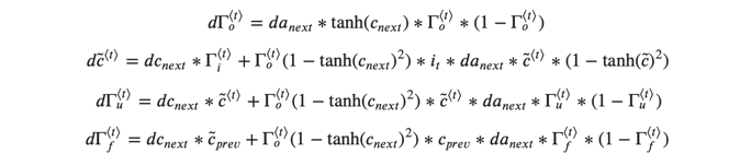
3.4.2 gate 导数
3.4.3 参数导数
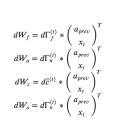
为了计算![]() , 您只需要在
, 您只需要在 ![]() 的 水平轴上(axis= 1) 求和,注意:您应该具有keep_dims = True选项。
的 水平轴上(axis= 1) 求和,注意:您应该具有keep_dims = True选项。
最后,您将针对先前的隐藏状态,先前的缓存状态和输入计算导数。
![]()
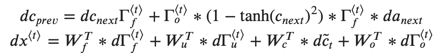
def lstm_cell_backward(da_next, dc_next, cache):
    """
    Implement the backward pass for the LSTM-cell (single time-step).

    Arguments:
    da_next -- Gradients of next hidden state, of shape (n_a, m)
    dc_next -- Gradients of next cell state, of shape (n_a, m)
    cache -- cache storing information from the forward pass

    Returns:
    gradients -- python dictionary containing:
                        dxt -- Gradient of input data at time-step t, of shape (n_x, m)
                        da_prev -- Gradient w.r.t. the previous hidden state, numpy array of shape (n_a, m)
                        dc_prev -- Gradient w.r.t. the previous memory state, of shape (n_a, m, T_x)
                        dWf -- Gradient w.r.t. the weight matrix of the forget gate, numpy array of shape (n_a, n_a + n_x)
                        dWi -- Gradient w.r.t. the weight matrix of the input gate, numpy array of shape (n_a, n_a + n_x)
                        dWc -- Gradient w.r.t. the weight matrix of the memory gate, numpy array of shape (n_a, n_a + n_x)
                        dWo -- Gradient w.r.t. the weight matrix of the save gate, numpy array of shape (n_a, n_a + n_x)
                        dbf -- Gradient w.r.t. biases of the forget gate, of shape (n_a, 1)
                        dbi -- Gradient w.r.t. biases of the update gate, of shape (n_a, 1)
                        dbc -- Gradient w.r.t. biases of the memory gate, of shape (n_a, 1)
                        dbo -- Gradient w.r.t. biases of the save gate, of shape (n_a, 1)
    """

    # Retrieve information from "cache"
    (a_next, c_next, a_prev, c_prev, ft, it, cct, ot, xt, parameters) = cache

    ### START CODE HERE ###
    # Retrieve dimensions from xt's and a_next's shape (≈2 lines)
    n_x, m = xt.shape
    n_a, m = a_next.shape

    # Compute gates related derivatives, you can find their values can be found by looking carefully at equations (7) to (10) (≈4 lines)
    dot = da_next * np.tanh(c_next) * ot * (1 - ot)
    dcct = (dc_next * it + ot * (1 - np.square(np.tanh(c_next))) * it * da_next) * (1 - np.square(cct))
    dit = (dc_next * cct + ot * (1 - np.square(np.tanh(c_next))) * cct * da_next) * it * (1 - it)
    dft = (dc_next * c_prev + ot * (1 - np.square(np.tanh(c_next))) * c_prev * da_next) * ft * (1 - ft)

    ## Code equations (7) to (10) (≈4 lines)
    ##dit = None
    ##dft = None
    ##dot = None
    ##dcct = None
    ##
    # Compute parameters related derivatives. Use equations (11)-(14) (≈8 lines)
    concat = np.concatenate((a_prev, xt), axis=0).T
    dWf = np.dot(dft, concat)
    dWi = np.dot(dit, concat)
    dWc = np.dot(dcct, concat)
    dWo = np.dot(dot, concat)
    dbf = np.sum(dft, axis=1, keepdims=True)
    dbi = np.sum(dit, axis=1, keepdims=True)
    dbc = np.sum(dcct, axis=1, keepdims=True)
    dbo = np.sum(dot, axis=1, keepdims=True)

    # Compute derivatives w.r.t previous hidden state, previous memory state and input. Use equations (15)-(17). (≈3 lines)
    da_prev = np.dot(parameters["Wf"][:, :n_a].T, dft) + np.dot(parameters["Wc"][:, :n_a].T, dcct) + np.dot(parameters["Wi"][:, :n_a].T, dit) + np.dot(parameters["Wo"][:, :n_a].T, dot)
    dc_prev = dc_next * ft + ot * (1-np.square(np.tanh(c_next))) * ft * da_next
    dxt = np.dot(parameters["Wf"][:, n_a:].T, dft) + np.dot(parameters["Wc"][:, n_a:].T, dcct) + np.dot(parameters["Wi"][:, n_a:].T, dit) + np.dot(parameters["Wo"][:, n_a:].T, dot)
    ### END CODE HERE ###

    # Save gradients in dictionary
    gradients = {"dxt": dxt, "da_prev": da_prev, "dc_prev": dc_prev, "dWf": dWf,"dbf": dbf, "dWi": dWi,"dbi": dbi,
                "dWc": dWc,"dbc": dbc, "dWo": dWo,"dbo": dbo}

    return gradients


np.random.seed(1)
xt = np.random.randn(3,10)
a_prev = np.random.randn(5,10)
c_prev = np.random.randn(5,10)
Wf = np.random.randn(5, 5+3)
bf = np.random.randn(5,1)
Wi = np.random.randn(5, 5+3)
bi = np.random.randn(5,1)
Wo = np.random.randn(5, 5+3)
bo = np.random.randn(5,1)
Wc = np.random.randn(5, 5+3)
bc = np.random.randn(5,1)
Wy = np.random.randn(2,5)
by = np.random.randn(2,1)

parameters = {"Wf": Wf, "Wi": Wi, "Wo": Wo, "Wc": Wc, "Wy": Wy, "bf": bf, "bi": bi, "bo": bo, "bc": bc, "by": by}

a_next, c_next, yt, cache = lstm_cell_forward(xt, a_prev, c_prev, parameters)

da_next = np.random.randn(5,10)
dc_next = np.random.randn(5,10)
gradients = lstm_cell_backward(da_next, dc_next, cache)
print("gradients[\"dxt\"][1][2] =", gradients["dxt"][1][2])
print("gradients[\"dxt\"].shape =", gradients["dxt"].shape)
print("gradients[\"da_prev\"][2][3] =", gradients["da_prev"][2][3])
print("gradients[\"da_prev\"].shape =", gradients["da_prev"].shape)
print("gradients[\"dc_prev\"][2][3] =", gradients["dc_prev"][2][3])
print("gradients[\"dc_prev\"].shape =", gradients["dc_prev"].shape)
print("gradients[\"dWf\"][3][1] =", gradients["dWf"][3][1])
print("gradients[\"dWf\"].shape =", gradients["dWf"].shape)
print("gradients[\"dWi\"][1][2] =", gradients["dWi"][1][2])
print("gradients[\"dWi\"].shape =", gradients["dWi"].shape)
print("gradients[\"dWc\"][3][1] =", gradients["dWc"][3][1])
print("gradients[\"dWc\"].shape =", gradients["dWc"].shape)
print("gradients[\"dWo\"][1][2] =", gradients["dWo"][1][2])
print("gradients[\"dWo\"].shape =", gradients["dWo"].shape)
print("gradients[\"dbf\"][4] =", gradients["dbf"][4])
print("gradients[\"dbf\"].shape =", gradients["dbf"].shape)
print("gradients[\"dbi\"][4] =", gradients["dbi"][4])
print("gradients[\"dbi\"].shape =", gradients["dbi"].shape)
print("gradients[\"dbc\"][4] =", gradients["dbc"][4])
print("gradients[\"dbc\"].shape =", gradients["dbc"].shape)
print("gradients[\"dbo\"][4] =", gradients["dbo"][4])
print("gradients[\"dbo\"].shape =", gradients["dbo"].shape)
输出结果:
gradients["dxt"][1][2] = 3.2305591151091884
gradients["dxt"].shape = (3, 10)
gradients["da_prev"][2][3] = -0.06396214197109246
gradients["da_prev"].shape = (5, 10)
gradients["dc_prev"][2][3] = 0.7975220387970015
gradients["dc_prev"].shape = (5, 10)
gradients["dWf"][3][1] = -0.14795483816449687
gradients["dWf"].shape = (5, 8)
gradients["dWi"][1][2] = 1.05749805522599
gradients["dWi"].shape = (5, 8)
gradients["dWc"][3][1] = 2.304562163687667
gradients["dWc"].shape = (5, 8)
gradients["dWo"][1][2] = 0.3313115952892111
gradients["dWo"].shape = (5, 8)
gradients["dbf"][4] = [0.18864637]
gradients["dbf"].shape = (5, 1)
gradients["dbi"][4] = [-0.40142491]
gradients["dbi"].shape = (5, 1)
gradients["dbc"][4] = [0.25587763]
gradients["dbc"].shape = (5, 1)
gradients["dbo"][4] = [0.13893342]
gradients["dbo"].shape = (5, 1)
3.5 LSTM RNN的后向传播
这部分与您在上面实现的rnn_backward函数非常相似。 首先,您将创建与返回变量相同维的变量。 然后,您将从头开始遍历所有时间步骤,并在每次迭代中调用为LSTM实现的一步功能。 然后,您将通过分别汇总参数来更新参数。 最后返回带有新渐变的字典。
def lstm_backward(da, caches):

    """
    Implement the backward pass for the RNN with LSTM-cell (over a whole sequence).

    Arguments:
    da -- Gradients w.r.t the hidden states, numpy-array of shape (n_a, m, T_x)
    dc -- Gradients w.r.t the memory states, numpy-array of shape (n_a, m, T_x)
    caches -- cache storing information from the forward pass (lstm_forward)

    Returns:
    gradients -- python dictionary containing:
                        dx -- Gradient of inputs, of shape (n_x, m, T_x)
                        da0 -- Gradient w.r.t. the previous hidden state, numpy array of shape (n_a, m)
                        dWf -- Gradient w.r.t. the weight matrix of the forget gate, numpy array of shape (n_a, n_a + n_x)
                        dWi -- Gradient w.r.t. the weight matrix of the update gate, numpy array of shape (n_a, n_a + n_x)
                        dWc -- Gradient w.r.t. the weight matrix of the memory gate, numpy array of shape (n_a, n_a + n_x)
                        dWo -- Gradient w.r.t. the weight matrix of the save gate, numpy array of shape (n_a, n_a + n_x)
                        dbf -- Gradient w.r.t. biases of the forget gate, of shape (n_a, 1)
                        dbi -- Gradient w.r.t. biases of the update gate, of shape (n_a, 1)
                        dbc -- Gradient w.r.t. biases of the memory gate, of shape (n_a, 1)
                        dbo -- Gradient w.r.t. biases of the save gate, of shape (n_a, 1)
    """

    # Retrieve values from the first cache (t=1) of caches.
    (caches, x) = caches
    (a1, c1, a0, c0, f1, i1, cc1, o1, x1, parameters) = caches[0]

    ### START CODE HERE ###
    # Retrieve dimensions from da's and x1's shapes (≈2 lines)
    n_a, m, T_x = da.shape
    n_x, m = x1.shape

    # initialize the gradients with the right sizes (≈12 lines)
    dx = np.zeros([n_x, m, T_x])
    da0 = np.zeros([n_a, m])
    da_prevt = np.zeros([n_a, m])
    dc_prevt = np.zeros([n_a, m])
    dWf = np.zeros([n_a, n_a + n_x])
    dWi = np.zeros([n_a, n_a + n_x])
    dWc = np.zeros([n_a, n_a + n_x])
    dWo = np.zeros([n_a, n_a + n_x])
    dbf = np.zeros([n_a, 1])
    dbi = np.zeros([n_a, 1])
    dbc = np.zeros([n_a, 1])
    dbo = np.zeros([n_a, 1])

    # loop back over the whole sequence
    for t in reversed(range(T_x)):
        # Compute all gradients using lstm_cell_backward
        gradients = lstm_cell_backward(da[:,:,t], dc_prevt,caches[t])
        # da_prevt, dc_prevt = gradients['da_prev'], gradients["dc_prev"]
        # Store or add the gradient to the parameters' previous step's gradient
        dx[:,:,t] = gradients['dxt']
        dWf = dWf + gradients['dWf']
        dWi = dWi + gradients['dWi']
        dWc = dWc + gradients['dWc']
        dWo = dWo + gradients['dWo']
        dbf = dbf + gradients['dbf']
        dbi = dbi + gradients['dbi']
        dbc = dbc + gradients['dbc']
        dbo = dbo + gradients['dbo']
    # Set the first activation's gradient to the backpropagated gradient da_prev.
    da0 = gradients['da_prev']

    ### END CODE HERE ###

    # Store the gradients in a python dictionary
    gradients = {"dx": dx, "da0": da0, "dWf": dWf,"dbf": dbf, "dWi": dWi,"dbi": dbi,
                "dWc": dWc,"dbc": dbc, "dWo": dWo,"dbo": dbo}

    return gradients

np.random.seed(1)
x = np.random.randn(3,10,7)
a0 = np.random.randn(5,10)
Wf = np.random.randn(5, 5+3)
bf = np.random.randn(5,1)
Wi = np.random.randn(5, 5+3)
bi = np.random.randn(5,1)
Wo = np.random.randn(5, 5+3)
bo = np.random.randn(5,1)
Wc = np.random.randn(5, 5+3)
bc = np.random.randn(5,1)

parameters = {"Wf": Wf, "Wi": Wi, "Wo": Wo, "Wc": Wc, "Wy": Wy, "bf": bf, "bi": bi, "bo": bo, "bc": bc, "by": by}

a, y, c, caches = lstm_forward(x, a0, parameters)

da = np.random.randn(5, 10, 4)
gradients = lstm_backward(da, caches)

print("gradients[\"dx\"][1][2] =", gradients["dx"][1][2])
print("gradients[\"dx\"].shape =", gradients["dx"].shape)
print("gradients[\"da0\"][2][3] =", gradients["da0"][2][3])
print("gradients[\"da0\"].shape =", gradients["da0"].shape)
print("gradients[\"dWf\"][3][1] =", gradients["dWf"][3][1])
print("gradients[\"dWf\"].shape =", gradients["dWf"].shape)
print("gradients[\"dWi\"][1][2] =", gradients["dWi"][1][2])
print("gradients[\"dWi\"].shape =", gradients["dWi"].shape)
print("gradients[\"dWc\"][3][1] =", gradients["dWc"][3][1])
print("gradients[\"dWc\"].shape =", gradients["dWc"].shape)
print("gradients[\"dWo\"][1][2] =", gradients["dWo"][1][2])
print("gradients[\"dWo\"].shape =", gradients["dWo"].shape)
print("gradients[\"dbf\"][4] =", gradients["dbf"][4])
print("gradients[\"dbf\"].shape =", gradients["dbf"].shape)
print("gradients[\"dbi\"][4] =", gradients["dbi"][4])
print("gradients[\"dbi\"].shape =", gradients["dbi"].shape)
print("gradients[\"dbc\"][4] =", gradients["dbc"][4])
print("gradients[\"dbc\"].shape =", gradients["dbc"].shape)
print("gradients[\"dbo\"][4] =", gradients["dbo"][4])
print("gradients[\"dbo\"].shape =", gradients["dbo"].shape)
输出结果:
gradients["dx"][1][2] = [-0.00173313  0.08287442 -0.30545663 -0.43281115]
gradients["dx"].shape = (3, 10, 4)
gradients["da0"][2][3] = -0.0959115019540047
gradients["da0"].shape = (5, 10)
gradients["dWf"][3][1] = -0.06981985612744011
gradients["dWf"].shape = (5, 8)
gradients["dWi"][1][2] = 0.10237182024854764
gradients["dWi"].shape = (5, 8)
gradients["dWc"][3][1] = -0.06249837949274524
gradients["dWc"].shape = (5, 8)
gradients["dWo"][1][2] = 0.04843891314443009
gradients["dWo"].shape = (5, 8)
gradients["dbf"][4] = [-0.0565788]
gradients["dbf"].shape = (5, 1)
gradients["dbi"][4] = [-0.15399065]
gradients["dbi"].shape = (5, 1)
gradients["dbc"][4] = [-0.29691142]
gradients["dbc"].shape = (5, 1)
gradients["dbo"][4] = [-0.29798344]
gradients["dbo"].shape = (5, 1)
恭喜你!
祝贺您完成此作业。 您现在了解了循环神经网络的工作原理!
让我们继续下一个练习,在该练习中,您将使用RNN来构建字符级语言模型。


 340
340


 被折叠的 条评论
为什么被折叠?
被折叠的 条评论
为什么被折叠?
 到【灌水乐园】发言


