【数据挖掘】决策树ID3算法Python实现

前言

文章内容为对数据挖掘实验作业的记录，如果您是为了作业而来看的这篇文章，还请不要无脑拷贝，本人编程能力较弱，代码写的并不优雅，注释尽可能写的详细了。

决策树算法

决策树是一类常见的机器学习方法.以二分类任务为例，我们希望从给定训练数据集学得一个模型用以对新示例进行分类，这个把样本分类的任务，可看作对“当前样本属于正类吗?”这个问题的“决策”或“判定 ”过程。
一般的，一棵决策树包含一个根结点、若干个内部结点和若干个叶结点，叶结点对应于决策结果，其他每个结点则对应于一个属性测试；每个结点包含的样本集合根据属性测试的结果被划分到子结点中；根结点包含样本全集。从根结点到每个叶结点的路径对应了一个判定测试序列。决策树学习的目的是为了产生一棵泛化能力强，即处理未见示例能力强的决策树，其基本流程遵循简单且直观的“分而治之"策略。

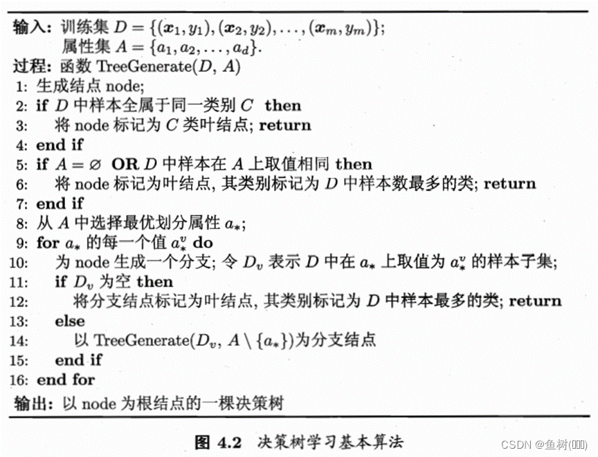
根据决策树的算法思想，如何选择最优划分属性至关重要，随着划分过程的不断进行，我们希望决策树的分支结点所包含的样本尽可能属于同一类别。
根据不同的划分规则，目前常见的决策树算法有ID3算法和C4.5算法

ID3算法

ID3算法主要根据信息增益对属性的重要程度进行划分


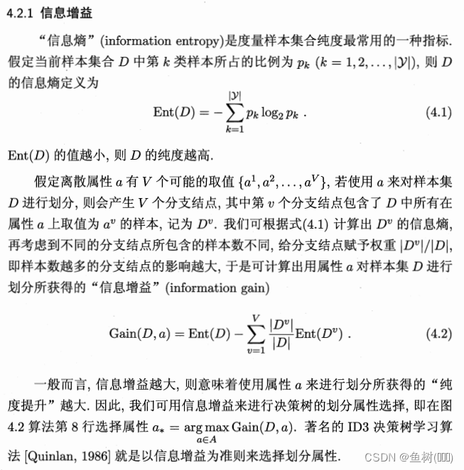
以上介绍出自著名机器学习书籍——西瓜书，这里只介绍了针对离散值的处理方式，但实际上，我们的样本数据更多的是连续性的数值，当遇到这种数据时，需要选择恰当的划分策略对数据进行划分，再应用ID3算法。

决策树算法进行分类的具体步骤

根据以上对决策树算法以及ID3、C4.5算法的分析，我们可以大致得到使用决策树对数据进行分类的具体步骤
(1) 数据预处理
(2) 对数据进行划分，计算各个属性的信息增益(ID3)或信息增益率(C4.5)
(3) 选择较大的信息增益或信息增益率对应的划分点构建决策树
(4) 使用样本数据对构建的决策树进行测试，得到正确率最大的决策树对应的深度
(5) 对陌生的数据进行分类预测

导入库

import numpy as np
import pandas as pd
from math import log
import matplotlib.pyplot as plt

分析样本数据

# 从本地读取样本数据集，这里选择前两种癌症数据进行分析
BLCA = pd.read_csv(r'数据集/BLCA/rna.csv')
KIRC = pd.read_csv(r'数据集/KIRC/rna.csv')
print(BLCA.shape)
print(KIRC.shape)

(3217, 400)
(3217, 489)

# 对数据进行转置，之后每行对应一个样本数据，每列对应一个属性
BLCASet = BLCA.T
BLCASet = BLCASet.iloc[1:,:].astype('float32')
KIRCSet = KIRC.T
KIRCSet = KIRCSet.iloc[1:,:].astype('float32')

# 插入一列数据用来标识不同的类别
BLCASet.insert(loc=3217, column=3217, value='BLCA')
KIRCSet.insert(loc=3217, column=3217, value='KIRC')

# 转为numpy类型方便处理
BLCASet = np.array(BLCASet)
KIRCSet = np.array(KIRCSet)

# 将两种癌症样本数据进行合并
DataSet = np.vstack((BLCASet,KIRCSet))

# 看一下合并后的样本数据规模
print(DataSet.shape)

(887, 3218)

# 对于连续的样本值，这里采取的划分方案是使用属性的最大最小值的平均值作为划分点
'''
至于为什么这种划分也会有效?
因为只要采取了某种划分策略对数据进行了划分，这个行为必然会带来一定的信息增益
"划分"所带来的信息增益就会给分类提供有用的信息
'''
maxlist = np.max(DataSet,axis=0)
minlist = np.min(DataSet,axis=0)
midlist = (maxlist[:-1]+minlist[:-1])/2
print(midlist)

[-0.3077172040939331 0.5645202994346619 0.038697242736816406 ...
 0.08328396081924438 0.25938647985458374 0.39306795597076416]

计算各个属性对应的信息增益

def I(s1, s2):
    '''
    计算信息熵
    '''
    t = s1+s2
    p1 = float(s1/t)
    p2 = float(s2/t)
    if p1*p2!=0:
        return -p1*log(p1,2)-p2*log(p2,2)
    else:
        if p1==0:
            return -p2*log(p2,2)
        else:
            return -p1*log(p1,2)

# 计算总熵
I_t = I(BLCASet.shape[0],KIRCSet.shape[0])

# 接下来为计算每种属性下的信息增益
row = DataSet.shape[0] # 获取样本行数
col = DataSet.shape[1] # 获取样本列数
Gain = [] # 存储样本属性的信息增益值
Sel = []  # 存储哪种分支可以确定类别，0表示>=,1表示<
Dec = []  # 存储可以确定的分支为哪一类，这里取值为"BLCA""KIRC"两种
S11 = []
S12 = []
S21 = []
S22 = []
for i in range(col-1): # 对样本每个属性求其信息增益
    data = DataSet[:,i] # 这一列的数据
    div = midlist[i]    # 这一列的划分点
    s11 = 0
    s12 = 0
    s21 = 0
    s22 = 0
    for j in range(row): # 对数据进行统计
        if data[j]>=div:
            if DataSet[j][-1] == 'BLCA':
                s11 = s11+1 # 大于等于划分点且属于BLCA的
            if DataSet[j][-1] == 'KIRC':
                s12 = s12+1 # 大于等于划分点且属于KIRC的
        else:
            if DataSet[j][-1] == 'BLCA':
                s21 = s21+1 # 小于划分点且属于BLCA的
            if DataSet[j][-1] == 'KIRC':
                s22 = s22+1 # 小于划分点且属于KIRC的
    I1 = I(s11, s12) # 计算熵I(s11,s12)
    I2 = I(s21, s22) # 计算熵I(s21,s22)
    S11.append(s11)
    S12.append(s12)
    S21.append(s21)
    S22.append(s22)
    Gain.append(I_t-((s11+s12)/len(data)*I1+(s21+s22)/len(data)*I2)) # 计算信息增益
    if I1<I2:
        Sel.append(0)
        if s11>s12:
            Dec.append('BLCA') # 表示如果一个数据大于等于划分点，将其判断为BLCA
        else:
            Dec.append('KIRC') # 表示如果一个数据大于等于划分点，将其判断为KIRC
    else:
        Sel.append(1)
        if s21>s22:
            Dec.append('BLCA') # 表示如果一个数据小于划分点，将其判断为BLCA
        else:
            Dec.append('KIRC') # 表示如果一个数据小于划分点，将其判断为KIRC

构建决策树

# 按照Gain中值的降序，对其下标进行排序
indexList = np.argsort(Gain)[::-1]

# 这里选择数据，利用数据与划分点的大小关系对其进行分类
def decisionTree(data, i):
    if i==len(data)-1:
        # print(f"到第{i}层可以做决策")
        if Sel[indexList[i-1]]==0:
            if S11[indexList[i-1]]>=S12[indexList[i-1]]:
                return 'KIRC'
            else:
                return 'BLCA'
        else:
            if S21[indexList[i-1]]>=S22[indexList[i-1]]:
                return 'KIRC'
            else:
                return 'BLCA'
    elif Sel[indexList[i]]==0 and data[i]>=midlist[indexList[i]]: # 大于等于可以决策
        # print(f"到第{i}层可以做决策")
        return Dec[indexList[i]]
    elif Sel[indexList[i]]==1 and data[i]<midlist[indexList[i]]: # 小于可以决策
        # print(f"到第{i}层可以做决策")
        return Dec[indexList[i]]
    else:
        return decisionTree(data, i+1)

计算决策树的正确率

# deep指定决策树的深度
deep = 6
data = np.array(DataSet[:,indexList[:deep]])
data = np.hstack((data,DataSet[:,-1].reshape(data.shape[0],1)))

total = data.shape[0]
corr = 0 
mis = 0
for i in range(0, total):
    global corr, mis
    res = decisionTree(data[i], 0)
    # print(res)
    if res == data[i][-1]:
        # print('正确')
        corr = corr + 1
    else:
        # print('错误')
        mis = mis + 1
print(f"{corr}/{total}")
print(f"深度为{deep}的决策树的正确率为{corr/total}")

879/887
深度为6的决策树的正确率为0.9909808342728298

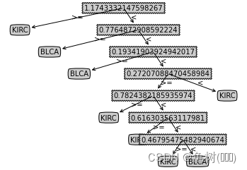
决策树的可视化

# 接下来为绘图的代码，唯独这里不是这一块不是原创，不过好像网上用的好像都一样?
def getNumLeafs(myTree):
    numLeafs = 0
    firstStr = list(myTree.keys())[0]
    secondDict = myTree[firstStr]
    for key in secondDict.keys():
        if type(secondDict[key]).__name__=='dict':
            numLeafs += getNumLeafs(secondDict[key])
        else:
            numLeafs += 1
    return numLeafs
def getTreeDepth(myTree):
    maxDepth = 0
    firstStr = list(myTree.keys())[0]
    secondDict = myTree[firstStr]
    for key in secondDict.keys():
        if type(secondDict[key]).__name__ == 'dict':
            thisDepth = 1 + getTreeDepth(secondDict[key])
        else:
            thisDepth = 1
        if thisDepth > maxDepth : maxDepth = thisDepth
    return maxDepth
decisionNode = dict(boxstyle = "sawtooth",fc="0.8")
leafNode = dict(boxstyle = "round4",fc="0.8")
arrow_args = dict(arrowstyle="<-")
def plotNode(nodeTxt,centerPt,parentPt,nodeType):
    createPlot.ax1.annotate(nodeTxt,xy=parentPt,\
    xycoords='axes fraction',xytext=centerPt,textcoords='axes fraction',\
    va="center",ha="center",bbox=nodeType,arrowprops=arrow_args)
def plotMidText(cntrPt,parentPt,txtString):
    xMid = (parentPt[0]-cntrPt[0])/2.0 + cntrPt[0]
    yMid = (parentPt[1]-cntrPt[1])/2.0 + cntrPt[1]
    createPlot.ax1.text(xMid,yMid,txtString)
def plotTree(myTree,parentPt,nodeTxt):
    numLeafs = getNumLeafs(myTree)
    depth = getTreeDepth(myTree)
    firstStr = list(myTree.keys())[0]
    cntrPt = (plotTree.xoff + (1.0 + float(numLeafs))/2.0/plotTree.totalW,\
              plotTree.yoff)
    plotMidText(cntrPt,parentPt,nodeTxt)
    plotNode(firstStr,cntrPt,parentPt,decisionNode)
    secondDict = myTree[firstStr]
    plotTree.yoff = plotTree.yoff - 1.0/plotTree.totalD
    for key in secondDict.keys():
        if type(secondDict[key]).__name__=='dict':
            plotTree(secondDict[key],cntrPt,str(key))
        else:
            plotTree.xoff = plotTree.xoff + 1.0 / plotTree.totalW
            plotNode(secondDict[key],(plotTree.xoff,plotTree.yoff),\
                     cntrPt,leafNode)
            plotMidText((plotTree.xoff,plotTree.yoff),cntrPt,str(key))
    plotTree.yoff = plotTree.yoff + 1.0 / plotTree.totalD
def createPlot(inTree):
    fig = plt.figure(1,facecolor='white')
    fig.clf()
    axprops = dict(xticks=[],yticks=[])
    createPlot.ax1 = plt.subplot(111,frameon=False,**axprops)
    plotTree.totalW = float(getNumLeafs(inTree))
    plotTree.totalD = float(getTreeDepth(inTree))
    plotTree.xoff = -0.5/plotTree.totalW
    plotTree.yoff = 1.0
    plotTree(inTree,(0.5,1.0),'')
    plt.show()

# 分析绘制树的代码可以知道，我们首先需要提供用“字典”表示的树
# 编写一个递归构建树的函数
def genInTree(deep,i):
    if i==deep:
        if Sel[indexList[i]]==0:
            if S11[indexList[i-1]]>=S12[indexList[i-1]]:
                return {midlist[indexList[i]]:{">=":"BLCA","<":"KIRC"}}
            else:
                return {midlist[indexList[i]]:{">=":"KIRC","<":"BLCA"}}
        else:
            if S21[indexList[i-1]]>=S22[indexList[i-1]]:
                return {midlist[indexList[i]]:{">=":"KIRC","<":"BLCA"}}
            else:
                return {midlist[indexList[i]]:{">=":"BLCA","<":"KIRC"}}
    else:
        if Sel[indexList[i]]==0:
            return {midlist[indexList[i]]:{">=":Dec[i],"<":genInTree(deep,i+1)}}
        else:
            return {midlist[indexList[i]]:{">=":genInTree(deep,i+1),"<":Dec[i]}}

# 其中deep为深度，也可以手动填
createPlot(genInTree(deep,0))

写在最后

这学期真是挺忙的 >_<，可以说算是百忙之中抽出时间来写这个选修课作业了ಥ_ಥ