数据科学与机器学习管道中预处理的重要性（二）：中心化、缩放和逻辑回归

http://geek.csdn.net/news/detail/75772

原文链接：The importance of preprocessing in data science and the machine learning pipeline II: centering, scaling and logistic regression 
作者：Hugo Bowne-Anderson 
译者：刘翔宇 审校：赵屹华 
责编：周建丁（zhoujd@csdn.net） 
未经许可，谢绝转载！

在本系列的第一篇文章中，我探索了机器学习（ML）分类任务中预处理的角色，深入了解了K近邻算法（k-NN）和红酒质量数据集。你见识到了通过对数值数据进行中心化和缩放，提升了k-NN多项模型性能指标（例如精度）。你同样学习到预处理不会凭空产生，而且它的价值只能在具体的预测机器学习管道的情形下来评判。然而，我们只见识到了预处理在一个模型（k-NN）中的重要性。在上面这种情况下，我们的模型表现有显著提高，但总是这样吗？未必！在这篇文章中，我将讨论缩放和中心化数值数据在另一种基本模型中的作用，也就是逻辑回归。你可能需要回顾上一篇文章以及/或者本文底部的词汇列表。我们将再次使用红酒质量数据集。本文所有的样例代码都由Python编写。如果你不熟悉Python，你可以参考我们的DataCamp课程。我将使用pandas库来处理数据以及scikit-learn来进行机器学习。

首先我将简要介绍回归，它可以用来预测数值变量和类别的值。我将介绍线性回归，逻辑回归，然后用后者来预测红酒质量。然后你会看到中心化和缩放是否会对回归模型有所帮助。

Python回归简介

线性回归Python实现

如上所述，回归通常用一个数值型变量预测另一个数值型变量。例如，在下面的代码中我们在波士顿住房数据（scikit-learn内置数据集）上使用了线性回归：在这里，自变量（x轴）是房间的数目，因变量（y轴）是房屋价格。

这种回归是如何工作的？简单来说，它的原理如下：我们希望将模型y=ax+b拟合数据 (xi ,yi )，也就是说，使用现有的数据，我们希望找到一个a和b的最优解。在普通的最小二乘（OLS，迄今为止最常见）公式中，假设了误差会在因变量中产生。出于这个原因，a和b的最优解由最小化误差得到： 

这种优化通常使用梯度下降算法来实现。下面我们在波士顿住房数据上使用简单的线性回归：

# Import necessary packages
import pandas as pd
%matplotlib inline
import matplotlib.pyplot as plt
plt.style.use('ggplot')
from sklearn import datasets
from sklearn import linear_model
import numpy as np
# Load data
boston = datasets.load_boston()
yb = boston.target.reshape(-1, 1)
Xb = boston['data'][:,5].reshape(-1, 1)
# Plot data
plt.scatter(Xb,yb)
plt.ylabel('value of house /1000 ($)')
plt.xlabel('number of rooms')
# Create linear regression object
regr = linear_model.LinearRegression()
# Train the model using the training sets
regr.fit( Xb, yb)
# Plot outputs
plt.scatter(Xb, yb,  color='black')
plt.plot(Xb, regr.predict(Xb), color='blue',
         linewidth=3)
plt.show()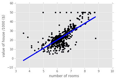

这种回归只捕获到了数据整体的增长趋势。我们仅使用了一个预测变量，不过我们可以使用更多预测变量，在模型中为每个预测变量使用n个系数a1,…,an。值得注意的是，系数ai的大小告诉我们对应变量与目标变量的相关程度。

逻辑回归Python实现

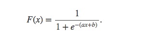
回归也可以用于分类问题。让人想到的第一个例子就是逻辑回归。在二分类（两个标签）中，我们可以把标签当做0和1。x表示预测变量，逻辑回归模型由下面的逻辑函数给出： 

这是一条sigmoidal（S形）曲线，如下图。对于任意x，如果F(x)<0.5，那么逻辑模型给出预测y=0，相反，如果F(X)>0.5，那么模型预测y=1。在有多个预测变量的情况下，我们有n个系数a1,…,an，每一个对应一个预测变量。在这种情况下，ai的大小告诉我们对应变量对预测变量的影响程度。

# Synthesize data
X1 = np.random.normal(size=150)
y1 = (X1 > 0).astype(np.float)
X1[X1 > 0] *= 4
X1 += .3 * np.random.normal(size=150)
X1= X1.reshape(-1, 1)
# Run the classifier
clf = linear_model.LogisticRegression()
clf.fit(X1, y1)
# Plot the result
plt.scatter(X1.ravel(), y1, color='black', zorder=20 , alpha = 0.5)
plt.plot(X1_ordered, clf.predict_proba(X1_ordered)[:,1], color='blue' , linewidth = 3)
plt.ylabel('target variable')
plt.xlabel('predictor variable')
plt.show()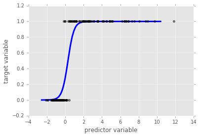

逻辑回归和数据缩放：红酒数据集

现在我们了解了逻辑回归的机制，接下来我们使用红酒数据集来实现一个逻辑回归分类器。我将导入数据然后画出目标变量（好/坏红酒）。

# Import necessary modules
from sklearn import linear_model
from sklearn.cross_validation import train_test_split
# Load data
df = pd.read_csv('http://archive.ics.uci.edu/ml/machine-learning-databases/wine-quality/winequality-red.csv ' , sep = ';')
X = df.drop('quality' , 1).values #drop target variable
y1 = df['quality'].values
y = y1 <= 5 # is the rating <= 5?
# plot histograms of original target variable
# and aggregated target variable
plt.figure(figsize=(20,5));
plt.subplot(1, 2, 1 );
plt.hist(y1);
plt.xlabel('original target value')
plt.ylabel('count')
plt.subplot(1, 2, 2);
plt.hist(y)
plt.xlabel('aggregated target value')
plt.show()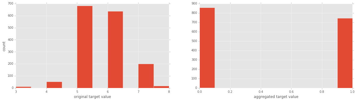

现在我们来运行下逻辑回归看看效果如何！

# Split the data into test and training sets
X_train, X_test, y_train, y_test = train_test_split(X, y, test_size=0.2, random_state=42)
#initial logistic regression model
lr = linear_model.LogisticRegression()
# fit the model
lr = lr.fit(X_train, y_train)
print('Logistic Regression score for training set: %f' % lr.score(X_train, y_train))
from sklearn.metrics import classification_report
y_true, y_pred = y_test, lr.predict(X_test)
print(classification_report(y_true, y_pred))

Logistic Regression score for training set: 0.752932
             precision    recall  f1-score   support

      False       0.78      0.74      0.76       179
       True       0.69      0.74      0.71       141

avg / total       0.74      0.74      0.74       320

非常不错，逻辑回归比k-NN（不管有没有数据缩放）效果要好。现在来对数据进行缩放然后再次使用逻辑回归：

from sklearn.preprocessing import scale
Xs = scale(X)
Xs_train, Xs_test, y_train, y_test = train_test_split(Xs, y, test_size=0.2, random_state=42)
lr_2 = lr.fit(Xs_train, y_train)
print('Scaled Logistic Regression score for test set: %f' % lr_2.score(Xs_test, y_test))
y_true, y_pred = y_test, lr_2.predict(Xs_test)
print(classification_report(y_true, y_pred))

Scaled Logistic Regression score for test set: 0.740625
             precision    recall  f1-score   support

      False       0.79      0.74      0.76       179
       True       0.69      0.74      0.72       141

avg / total       0.74      0.74      0.74       320

这非常有意思！使用数据缩放后，逻辑回归的性能并没有提升。为什么会这样，特别是我们看到在k-NN上使用缩放性能大幅提升之后？其原因在于，如果有大范围的预测变量，它们不会影响目标变量，回归算法会将相应的系数ai调小，这样它们就不会对预测有太大影响。k-NN没有这种内置的策略，所以我们需要缩放数据。

在下一篇文章中，我将揭秘k-NN和逻辑回归中使用中心化和缩放产生的巨大不同，我将对数据集进行合成，加入噪声数据，看看使用不同强度的噪声，中心化和缩放会对这两个模型性能有多大影响。

在下面的交互式窗口中，你可以玩转数据。你可以通过设定sc=True来缩放数据。然后运行整个脚本来生成逻辑回归模型的精度报告和分类报告。

# Set sc = True if you want to scale your features
sc = False

# Load data
df = pd.read_csv('http://archive.ics.uci.edu/ml/machine-learning-databases/wine-quality/winequality-red.csv ' , sep = ';')
X = df.drop('quality' , 1).values # drop target variable

# Here we scale, if desired
if sc == True:
X = scale(X)

# Target value
y1 = df['quality'].values # original target variable
y = y1 <= 5 # new target variable: is the rating <= 5?

# Split the data into a test set and a training set
X_train, X_test, y_train, y_test = train_test_split(X, y, test_size=0.2, random_state=42)

# Train logistic regression model and print performance on the test set
lr = linear_model.LogisticRegression()
lr = lr.fit(X_train, y_train)
print('Logistic Regression score for training set: %f' % lr.score(X_train, y_train))
y_true, y_pred = y_test, lr.predict(X_test)
print(classification_report(y_true, y_pred))

<script.py> output:
    Logistic Regression score for training set: 0.752932
                 precision    recall  f1-score   support

          False       0.78      0.74      0.76       179
           True       0.69      0.74      0.71       141

    avg / total       0.74      0.74      0.74       320

术语表

监督式学习（Supervised learning）：使用预测变量推断目标变量。比如从“年龄”，“性别”和“是否吸烟”这样的预测变量中推断目标变量“患心脏病”。

分类任务（Classfication task）：如果目标变量属于类别（比如“点击”或“不是”，“恶性”或“良性”肿瘤），那么这种监督式学习任务就是一个分类任务。

回归任务（Regression task）：如果目标变量属于连续变化变量（比如房屋价格）或是有序的分类变量，比如“红酒质量级别”，那么这种监督式学习任务就是一个回归任务。

K近邻（k-Nearest Neighbors）：分类任务的一种算法，一个数据点的标签由离它最近的k个质心投票决定。

预处理：数据科学家会使用的任何操作，将原始数据转换成更适合他们工作的形式。例如，在对推特数据进行情感分析之前，你可能想去掉所有的HTML标签，空格，展开缩写词，将推文分割成词汇列表。

中心化和缩放：这都是数值数据预处理方式，这些数据包含数字，而不是类别或字符；对一个变量进行中心化就是减去所有数据点的平均值，让新变量的平均值为0；缩放变量就是对每个数据点乘以一个常数来改变数据的范围。想知道这些操作的重要性，参见全文以及案例。