B站台大MATLAB教学视频自学整理---回归与内插【13】

*B站视频链接：**台大郭彦甫教授的教学视频

1 多项式拟合

• polyfit(x ,y,n) : 多项式曲线拟合,n为多项式的最高次幂。

练习1

%% 练习1
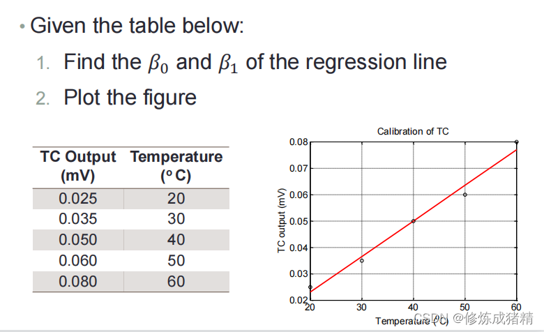
x = [0.025 0.035 0.050 0.060 0.080];
y = [20    30    40    50    60];
fit = polyfit(x,y,1);
xfit = x(1):0.001:x(end);
yfit = fit(1)*xfit + fit(2);
t=plot(x,y,'bo',xfit,yfit,'r');
set(t,'LineWidth',2)
set(gca,'FontSize',14)
xlabel('Temperature(°C)')
ylabel('TC output(mV)')
title('Calibration of TC')

1.1 x和y是否是线性关系

• scatter(x,y) : 画散点图
• corrcoef(x,y) : 相关系数（correlation coefficient ）,返回x和y之间的关系系数（$-1⩽r⩽1$），

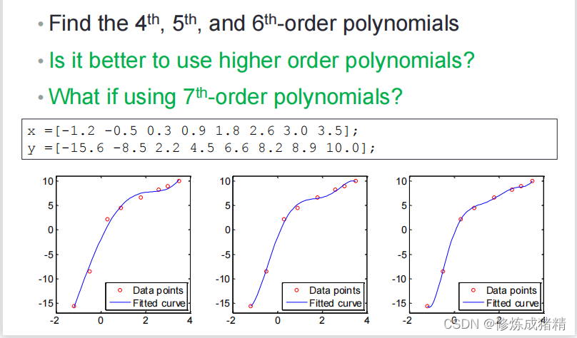
1.2 高阶多项式拟合

练习2

%% 练习2
x = [-1.2  -0.5 0.3 0.9 1.8 2.6 3.0 3.5 ];
y = [-15.6 -8.5 2.2 4.5 6.6 8.2 8.9 10.0];
figure('Position',[50 50 1500 400]);
for i=1:3
    subplot(1,3,i);
    p = polyfit(x,y,i+3);
    xfit = x(1):0.1:x(end);
    yfit = polyval(p,xfit);
    plot(x,y,'ro',xfit,yfit,'b')
    set(gca,'FontSize',14)
    ylim([-17,11])
    legend('data points','curve fit')
end

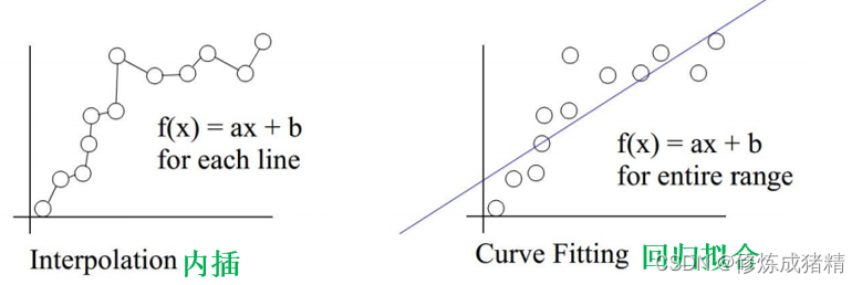
1.3 回归

• regress（）：多重线回归

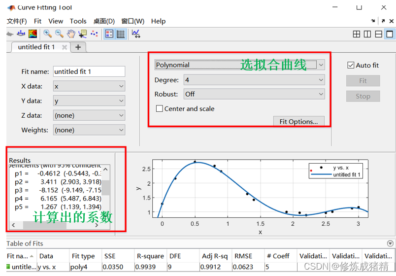
1.4非线性拟合

• cftool() : matlab 拟合工具箱
• 

2 内插

• interpre1() : 线性内插
• pchip() :
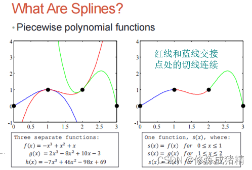
• spline() : 三次样条插值 cubic spline
• mkpp() :
  
  练习3
  

%% 练习3
x = 0:0.01:2.25;
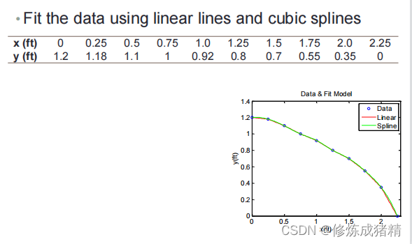
x_ft = [0    0.25  0.5  0.75   1.0   1.25  1.5  1.75  2.0  2.25];
y_ft = [1.2  1.18  1.1    1    0.92   0.8  0.7  0.55  0.35  0  ];
y_linear = interp1(x_ft,y_ft,x);
y_spline = spline(x_ft,y_ft,x);
plot(x_ft,y_ft,'bo',x,y_linear,'-r',x,y_spline,'-g')
h = legend('Data','Linear','Spline');
set(h,'FontName','Times New Roman')
xlabel('x(ft)')
ylabel('y(ft)')
title('Data & Fit Model')
box on

• interp2() : 二维内插
• interp2(…,‘curbic’) = cubic spline: