


机器学习——Iris的数据处理
详细内容见知乎:https://zhuanlan.zhihu.com/p/26802995
代码链接:https://pan.baidu.com/s/11T-StES9iY_bxqeKiQD9tw 密码:3tw5
Irisdemo.py代码:
# Load libraries
import pandas
from pandas.tools.plotting import scatter_matrix #导入散点图矩阵包
import matplotlib.pyplot as plt
from sklearn import datasets
import csv
import numpy as np
import xlrd
###################################################
# 读取csv文件,返回列表,tolist() & np.array()
def csvfile_load(filename = '待读取.csv'):
csvfile = open(filename, encoding = 'utf-8')
data = csv.reader(csvfile)
dataset = []
for line in data:
dataset.append(line)
csvfile.close()
return dataset
# 读取xlsx文件,返回列表,tolist() & np.array()
def xlsxfileload(filename = '待读取.xlsx'):
dataset = []
workbook = xlrd.open_workbook(filename)
table = workbook.sheets()[0]
for row in range(table.nrows):
dataset.append(table.row_values(row))
return dataset
######################################################
dataset = pandas.read_csv('iris.csv') # 读入csv文件
# dataset = np.array(xlsxfileload('iris.xlsx'))
#
# # Load dataset
# url = "https://archive.ics.uci.edu/ml/machine-learning-databases/iris/iris.data" #数据集的下载网址
# names = ['sepal-length', 'sepal-width', 'petal-length', 'petal-width', 'class'] #添加抬头
# dataset = pandas.read_csv(url, names=names) #读取csv数据
# dataset.to_csv("iris.csv",index=False,sep=',') #保存数据集为csv文件
# iris = datasets.load_iris()
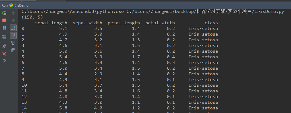
print(dataset.shape)
# head
print(dataset.head(150)) # print(dataset.describe())
# class distribution
print(dataset.groupby('class').size())
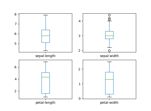
# box and whisker plots
dataset.plot(kind='box', subplots=True, layout=(2,2), sharex=False, sharey=False)
plt.show()
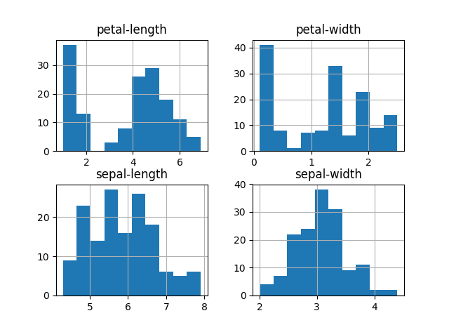
# histograms
dataset.hist()
plt.show()
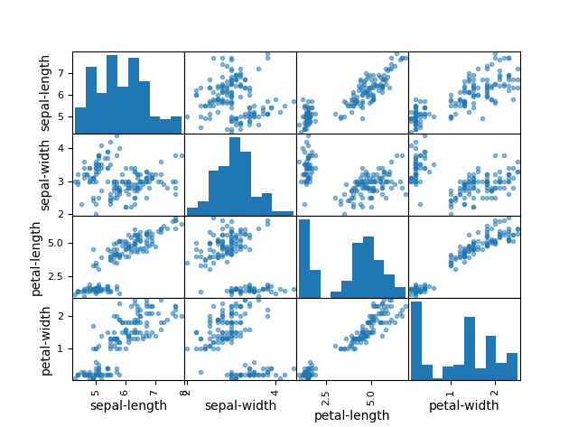
# scatter plot matrix
scatter_matrix(dataset)
plt.show()
print("End!")运行结果为:

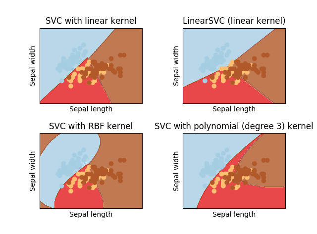
Iris_SVM.py:
import numpy as np
import matplotlib.pyplot as plt
from sklearn import svm, datasets

# 导入数据集
iris = datasets.load_iris()
X = iris.data[:, :2]  # 只取前两维特征
y = iris.target

h = .02  # 网格中的步长

# 创建支持向量机实例,并拟合出数据
C = 1.0  # SVM正则化参数
svc = svm.SVC(kernel='linear', C=C).fit(X, y) # 线性核
rbf_svc = svm.SVC(kernel='rbf', gamma=0.7, C=C).fit(X, y) # 径向基核
poly_svc = svm.SVC(kernel='poly', degree=3, C=C).fit(X, y) # 多项式核
lin_svc = svm.LinearSVC(C=C).fit(X, y) #线性核

# 创建网格,以绘制图像
x_min, x_max = X[:, 0].min() - 1, X[:, 0].max() + 1
y_min, y_max = X[:, 1].min() - 1, X[:, 1].max() + 1
xx, yy = np.meshgrid(np.arange(x_min, x_max, h),
                     np.arange(y_min, y_max, h))

# 图的标题
titles = ['SVC with linear kernel',
          'LinearSVC (linear kernel)',
          'SVC with RBF kernel',
          'SVC with polynomial (degree 3) kernel']


for i, clf in enumerate((svc, lin_svc, rbf_svc, poly_svc)):
    # 绘出决策边界,不同的区域分配不同的颜色
    plt.subplot(2, 2, i + 1) # 创建一个2行2列的图,并以第i个图为当前图
    plt.subplots_adjust(wspace=0.4, hspace=0.4) # 设置子图间隔

    Z = clf.predict(np.c_[xx.ravel(), yy.ravel()]) #将xx和yy中的元素组成一对对坐标,作为支持向量机的输入,返回一个array

    # 把分类结果绘制出来
    Z = Z.reshape(xx.shape) #(220, 280)
    plt.contourf(xx, yy, Z, cmap=plt.cm.Paired, alpha=0.8) #使用等高线的函数将不同的区域绘制出来

    # 将训练数据以离散点的形式绘制出来
    plt.scatter(X[:, 0], X[:, 1], c=y, cmap=plt.cm.Paired)
    plt.xlabel('Sepal length')
    plt.ylabel('Sepal width')
    plt.xlim(xx.min(), xx.max())
    plt.ylim(yy.min(), yy.max())
    plt.xticks(())
    plt.yticks(())
    plt.title(titles[i])

plt.show()
运行结果为:
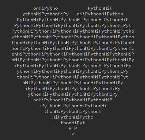
最后,娱乐一下,给一个看到的一行代码能干啥!!!
print('\n'.join([''.join([('HiPython'[(x-y)%len('HiPython')]if((x*0.05)**2+(y*0.1)**2-1)**3-(x*0.05)**2*(y*0.1)**3<=0 else' ')for x in range(-32,32)])for y in range(17,-17,-1)]))
运行结果为:


 4751
4751

 被折叠的 条评论
为什么被折叠?
被折叠的 条评论
为什么被折叠?
 到【灌水乐园】发言


