深度详细理解ConvNeXt网络代码（结合代码）

置顶 zqx951102

已于 2022-11-08 15:00:20 修改

阅读量4.3k

点赞数 8

分类专栏：目标检测算法论文文章标签：网络深度学习计算机视觉

于 2022-11-08 11:00:29 首次发布

本文链接：https://blog.csdn.net/zqx951102/article/details/127746625

版权

论文同时被 3 个专栏收录

46 篇文章

订阅专栏

算法

32 篇文章

订阅专栏

目标检测

9 篇文章

订阅专栏

1.简介

2.ConvNeXt的设计与实验

2.1 macro design（大的结构上的设计）

2.1.1 Changing stage compute ratio（改变每个stage的堆叠次数）

2.1.2 Changing stem to “Patchify”（stem为最初的下采样模块，改为与swin相似的patch卷积进行下采样）

2.2 ResNeXt（参考ResNeXt）

2.2.1 depth conv（普通卷积改为DW 卷积）

2.2.2 width（增加每个stage网络的深度）

2.3 inverted bottleneck

2.3.1 inverting dims（bottleneck由Resnet中两头粗中间细改为了类似Mobilenetv2中两头细中间粗的结构）

2.4 large kerner size（增加卷积核大小）

2.4.1 Moving up depthwise conv layer（将bottleneck中DW卷积模块上移）

2.4.2 Increasing the kernel size（增大DW卷积的卷积核大小）

2.5 various layer-wise micro designs（微小结构的设计）

2.5.1 Replacing ReLU with GELU（激活函数的改变）

2.5.2 Fewer activation functions（使用更少的激活函数，仅在DW卷积后的全连接层使用激活函数）

编辑

2.5.3 Fewer normalization layers（将BN替换为LN，并且只在DW卷积后使用LN）

2.5.4 Substituting BN with LN（将BN替换为LN）

2.5.5 Separate downsampling layers（将Resnet中在bottleneck中进行下采样改为使用单独的下采样层）

3. ConvNeXt 的版本

4.ConvNeXt的整体结构

5. ConvNeXt网络模型代码

1.简介

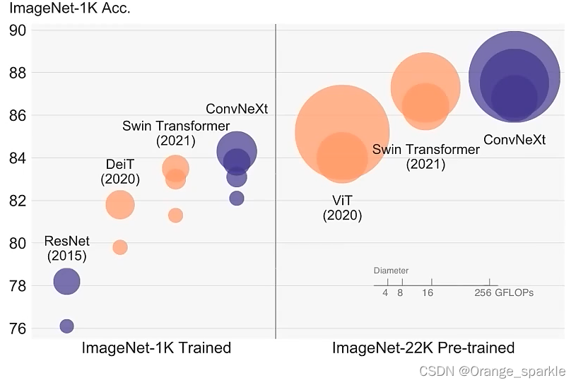
摘要：视觉识别的“咆哮的二十世纪”开始于ViT的引入，ViT迅速的取代卷积网络成为图像分类模型的SOTA。当普通的ViT在通用计算机视觉任务中比如目标检测和语义分割当中遇到困难时，hierarchical Transformers，比如swin transformer重新引入了几个卷积中的先验知识，使得transformer作为通用的计算机视觉的backbone实际上是可行的，并且展示了在各种视觉任务中的卓越的性能。然而，许多混合方法的效率任然大量的依靠Transformer自身固有的优势，而不是卷积自身的归纳偏置。在这篇工作中，复查了设计空间并且验证了限制纯卷积网络的实现的是什么原因。逐渐“现代化”一个标准的ResNet向着ViT的方向设计，并且发现了几个关键的参数，随着方法的不同而贡献了不同的性能提升。这个探索的结果是一个称为ConvNeXt的纯卷积网络。完全从标准的卷积网络构建的ConvNeXt，从精度和泛化性角度来说，完全不逊色于Transformer，在imagenet上以top-1中87.8%的精度，并且在COCO检测和ADE20K上的性能都优于swin Transformer，并且还维持了标准卷积网络的简单和有效性。

卷积在计算视觉领域的统治力不是一个巧合，滑动窗口策略是固有的对于视觉处理来说，归纳偏置和平移不变性能使Convnet非常适用在计算机视觉的应用上。

ViT遇到的困难是通过swin transformer来解决的，而swin Transformer恰恰是引入了卷积中的滑动窗口的，所以说明卷积是非常重要的，而我们可以将Transformer的优势来引入到卷积网络当中。然而，以前的尝试是有代价的，要么就是非常贵，要么就是将系统设计的非常复杂。讽刺的是，卷积网络已经满足了这些所需的属性，尽管是直接简单的、不加修饰的方法。似乎ConvNets失去动力的唯一原因是(分级)Transformer在许多视觉任务中超过了它们，而性能差异通常归因于Transformer的优越尺度行为，其中多头自注意是关键组件。

文章的中心就是探讨一个问题：How do design decisions in Transformers impact ConvNets’ performance?

ConvNeXt网络本身没有什么亮点，全是应用的现有的方法来进行网络的调整，特别是大量细节的设计都是参考了swin transformer的网络结构的。并且ConvNeXt是以ResNet50网络为backbone来进行调整的，所以ConvNeXt的网络结构非常简单，一目了然，理解起来也是非常容易的。并且不仅精度比swin Transformer高，推理速度还快。

综合来说，ConvNeXt是一个非常好的文章。这里放上我看到的一个网友对ConvNeXt网络的评价。

“感觉这篇论文的思路是照着swin-transformer的结构靠拢的，可以明显的看出来很多设计都是损于推理速度的，比如激活函数的选择，组卷积的使用，分支数量的增加，这是一篇很不错的论文，其给出了详细的设计思路同时又留下了很多针对于推理速度的改进空间，我觉得现在卷积神经网络的另一个方向可以研究等效，即repvgg论文中使用的，训练时采用残差结构提高精度，而推理时转化为单分支结构极大的提高推理速度，因为各大ai芯片以及nvidia对3*3卷积的优化的非常的好，以我个人浅薄的认知而言，卷积神经网络的瓶颈还远远没有达到，未来在推理速度的研究方面，卷积神经网络因为其简单的结构很有可能会再次走在transformer的前面。”

2.ConvNeXt的设计与实验

作者以通过ViT的训练策略训练的Resnet50网络（精度78.8）作为基准网络进行调整，最后能达到82.0的准确率（高于swin-T的81.3），说明将swin Transformer的结构和训练策略应用到Resnet上是很有效果的。

我们知道，训练策略也会影响到最终的模型性能，ViT不仅带来了新的模块和结构的设计，还带来了不同的训练技巧。因此，第一步就是用ViT的训练策略来训练ResNet50/200。在这篇文章中，用的训练策略更接近于DeiT和Swin Transformer的训练策略。

1）训练次数由之前的90个epoch扩大到150个epoch。

2）用了AdamW优化器

3）用了许多数据增强的技术，比如：Mixup、Cutmix、RandAugment、Random Erasing

4）用了正则化策略，有Stochastic Depth和Label Smoothing

通过使用以上这些训练策略，ResNet的准确率由76.1%提升到了78.8%（+2.7%）。

ConvNeX网络的改进主要有以下五个方面：

在这里插入图片描述

2.1 macro design（大的结构上的设计）
- 2.1.1 Changing stage compute ratio（改变每个stage的堆叠次数）
  
  在原ResNet网络中，一般conv4_x（即stage3）堆叠的block的次数是最多的。ResNet50中stage1到stage4堆叠block的次数是(3, 4, 6, 3)比例大概是1:1:2:1，但在Swin Transformer中，比如Swin-T的比例是1:1:3:1，Swin-L的比例是1:1:9:1。很明显，在Swin Transformer中，stage3堆叠block的占比更高。所以作者就将ResNet50中的stage中的堆叠次数由(3, 4, 6, 3)调整成(3, 3, 9, 3)，和Swin-T拥有相似的FLOPs。进行调整后，准确率由78.8%提升到了79.4%。
- 2.1.2 Changing stem to “Patchify”（stem为最初的下采样模块，改为与swin相似的patch卷积进行下采样）
  
  在之前的卷积神经网络中，一般最初的下采样模块stem一般都是通过一个卷积核大小为7x7步距为2的卷积层以及一个步距为2的最大池化下采样共同组成，高和宽都下采样4倍。但在Transformer模型中一般都是通过一个卷积核非常大且相邻窗口之间没有重叠的（即stride等于kernel_size）卷积层进行下采样。比如在Swin Transformer中采用的是一个卷积核大小为4x4步距为4的卷积层构成patchify，同样是下采样4倍。所以作者将ResNet中的stem也换成了和Swin Transformer一样的patchify。替换后准确率从79.4% 提升到79.5%，并且FLOPs也降低了一点。
2.2 ResNeXt（参考ResNeXt）
- 2.2.1 depth conv（普通卷积改为DW 卷积）
  
  借鉴了ResNeXt中的组卷积grouped convolution，因为ResNeXt相比普通的ResNet而言在FLOPs以及accuracy之间做到了更好的平衡。而作者采用的是更激进的depthwise convolution，即group数和通道数channel相同。这样做的另一个原因是作者认为depthwise convolution和self-attention中的加权求和操作很相似。
  
  DW卷积能对空间上的信息进行提取，1x1卷积能对通道上的信息进行提取。
- 2.2.2 width（增加每个stage网络的深度）
  
  将最初的通道数由64调整成96和Swin Transformer保持一致，增加了FLOPs（5.3G），最终准确率达到了80.5%。
2.3 inverted bottleneck
- 2.3.1 inverting dims（bottleneck由Resnet中两头粗中间细改为了类似Mobilenetv2中两头细中间粗的结构）
  
  作者认为Transformer block中的MLP模块非常像MobileNetV2中的Inverted Bottleneck模块，即两头细中间粗。作者采用Inverted Bottleneck模块后，在较小的模型上准确率由80.5%提升到了80.6%，在较大的模型上准确率由81.9%提升到82.6%。
2.4 large kerner size（增加卷积核大小）
- 2.4.1 Moving up depthwise conv layer（将bottleneck中DW卷积模块上移）
  
  将depthwise conv模块上移，原来是1x1 conv -> depthwise conv -> 1x1 conv，现在变成了depthwise conv -> 1x1 conv -> 1x1 conv。这么做是因为在Transformer中，MSA模块是放在MLP模块之前的，所以这里进行效仿，将depthwise conv上移。这样改动后，准确率虽然下降到了79.9%，但同时FLOPs也减小了。
- 2.4.2 Increasing the kernel size（增大DW卷积的卷积核大小）
  
  作者将depthwise conv的卷积核大小由3x3改成了7x7（和Swin Transformer一样），当然作者也尝试了其他尺寸，包括3, 5, 7, 9, 11发现取到7时准确率就达到了饱和。并且准确率从79.9% (3×3) 增长到 80.6% (7×7)。
2.5 various layer-wise micro designs（微小结构的设计）
- 2.5.1 Replacing ReLU with GELU（激活函数的改变）
  
  在Transformer中激活函数基本用的都是GELU，而在卷积神经网络中最常用的是ReLU，于是作者又将激活函数替换成了GELU，替换后发现准确率没变化。
- 2.5.2 Fewer activation functions（使用更少的激活函数，仅在DW卷积后的全连接层使用激活函数）
  
  使用更少的激活函数。在卷积神经网络中，一般会在每个卷积层或全连接后都接上一个激活函数。但在Transformer中并不是每个模块后都跟有激活函数，比如MLP中只有第一个全连接层后跟了GELU激活函数。接着作者在ConvNeXt Block中也减少激活函数的使用，如下图所示，减少后发现准确率从80.6%增长到81.3%。
- 2.5.3 Fewer normalization layers（将BN替换为LN，并且只在DW卷积后使用LN）
  
  在Transformer中，Normalization使用的也比较少，接着作者也减少了ConvNeXt Block中的Normalization层，只保留了depthwise conv后的Normalization层。此时准确率已经达到了81.4%，已经超过了Swin-T。
- 2.5.4 Substituting BN with LN（将BN替换为LN）
  
  在Transformer中基本都用的Layer Normalization（LN），因为最开始Transformer是应用在NLP领域的，BN又不适用于NLP相关任务。接着作者将BN全部替换成了LN，发现准确率还有小幅提升达到了81.5%。
- 2.5.5 Separate downsampling layers（将Resnet中在bottleneck中进行下采样改为使用单独的下采样层）
  
  在ResNet网络中stage2-stage4的下采样都是通过将主分支上3x3的卷积层步距设置成2，捷径分支上1x1的卷积层步距设置成2进行下采样的。但在Swin Transformer中是通过一个单独的Patch Merging实现的。接着作者就为ConvNext网络单独使用了一个下采样层，就是通过一个Laryer Normalization加上一个卷积核大小为2步距为2的卷积层构成。更改后准确率就提升到了82.0%，超过了Swin-T的81.3%。

3. ConvNeXt 的版本

对于ConvNeXt网络，作者提出了T/S/B/L四个版本，计算复杂度刚好和Swin Transformer中的T/S/B/L相似。

这四个版本的配置如下：

ConvNeXt-T: C = (96, 192, 384, 768), B = (3, 3, 9, 3)
ConvNeXt-S: C = (96, 192, 384, 768), B = (3, 3, 27, 3)
ConvNeXt-B: C = (128, 256, 512, 1024), B = (3, 3, 27, 3)
ConvNeXt-L: C = (192, 384, 768, 1536), B = (3, 3, 27, 3)
ConvNeXt-XL: C = (256, 512, 1024, 2048), B = (3, 3, 27, 3)
其中C代表4个stage中输入的通道数，B代表每个stage重复堆叠block的次数。

4.ConvNeXt的整体结构

下图是另一个博主画的网络结构图，博文链接(6条消息) ConvNeXt网络详解_太阳花的小绿豆的博客-CSDN博客

ConvNeXt Block会发现其中还有一个Layer Scale操作（论文中并没有提到），其实它就是将输入的特征层乘上一个可训练的参数，该参数就是一个向量，元素个数与特征层channel相同，即对每个channel的数据进行缩放。

在这里插入图片描述

5. ConvNeXt网络模型代码

"""
original code from facebook research:
https://github.com/facebookresearch/ConvNeXt
"""

import torch
import torch.nn as nn
import torch.nn.functional as F


def drop_path(x, drop_prob: float = 0., training: bool = False):
    """Drop paths (Stochastic Depth) per sample (when applied in main path of residual blocks).
    This is the same as the DropConnect impl I created for EfficientNet, etc networks, however,
    the original name is misleading as 'Drop Connect' is a different form of dropout in a separate paper...
    See discussion: https://github.com/tensorflow/tpu/issues/494#issuecomment-532968956 ... I've opted for
    changing the layer and argument names to 'drop path' rather than mix DropConnect as a layer name and use
    'survival rate' as the argument.
    """
    if drop_prob == 0. or not training:
        return x
    keep_prob = 1 - drop_prob
    shape = (x.shape[0],) + (1,) * (x.ndim - 1)  # work with diff dim tensors, not just 2D ConvNets
    random_tensor = keep_prob + torch.rand(shape, dtype=x.dtype, device=x.device)
    random_tensor.floor_()  # binarize
    output = x.div(keep_prob) * random_tensor
    return output


class DropPath(nn.Module):
    """Drop paths (Stochastic Depth) per sample  (when applied in main path of residual blocks).
    """

    def __init__(self, drop_prob=None):
        super(DropPath, self).__init__()
        self.drop_prob = drop_prob

    def forward(self, x):
        return drop_path(x, self.drop_prob, self.training)


class LayerNorm(nn.Module):
    r""" LayerNorm that supports two data formats: channels_last (default) or channels_first.
    The ordering of the dimensions in the inputs. channels_last corresponds to inputs with
    shape (batch_size, height, width, channels) while channels_first corresponds to inputs
    with shape (batch_size, channels, height, width).
    官方实现的LN是默认对最后一个维度进行的，这里是对channel维度进行的，所以单另设一个类。
    """

    def __init__(self, normalized_shape, eps=1e-6, data_format="channels_last"):
        super().__init__()
        self.weight = nn.Parameter(torch.ones(normalized_shape), requires_grad=True)
        self.bias = nn.Parameter(torch.zeros(normalized_shape), requires_grad=True)
        self.eps = eps
        self.data_format = data_format
        if self.data_format not in ["channels_last", "channels_first"]:
            raise ValueError(f"not support data format '{self.data_format}'")
        self.normalized_shape = (normalized_shape,)

    def forward(self, x: torch.Tensor) -> torch.Tensor:
        if self.data_format == "channels_last":
            return F.layer_norm(x, self.normalized_shape, self.weight, self.bias, self.eps)
        elif self.data_format == "channels_first":
            # [batch_size, channels, height, width]
            mean = x.mean(1, keepdim=True)
            var = (x - mean).pow(2).mean(1, keepdim=True)
            x = (x - mean) / torch.sqrt(var + self.eps)
            x = self.weight[:, None, None] * x + self.bias[:, None, None]
            return x


class Block(nn.Module):
    r""" ConvNeXt Block. There are two equivalent implementations:
    (1) DwConv -> LayerNorm (channels_first) -> 1x1 Conv -> GELU -> 1x1 Conv; all in (N, C, H, W)
    (2) DwConv -> Permute to (N, H, W, C); LayerNorm (channels_last) -> Linear -> GELU -> Linear; Permute back
    We use (2) as we find it slightly faster in PyTorch
    Args:
        dim (int): Number of input channels.
        drop_rate (float): Stochastic depth rate. Default: 0.0
        layer_scale_init_value (float): Init value for Layer Scale. Default: 1e-6.
    """

    def __init__(self, dim, drop_rate=0., layer_scale_init_value=1e-6):
        super().__init__()
        self.dwconv = nn.Conv2d(dim, dim, kernel_size=7, padding=3, groups=dim)  # depthwise conv
        self.norm = LayerNorm(dim, eps=1e-6, data_format="channels_last")
        self.pwconv1 = nn.Linear(dim, 4 * dim)  # pointwise/1x1 convs, implemented with linear layers
        self.act = nn.GELU()
        self.pwconv2 = nn.Linear(4 * dim, dim)
        # layer scale
        self.gamma = nn.Parameter(layer_scale_init_value * torch.ones((dim,)),
                                  requires_grad=True) if layer_scale_init_value > 0 else None
        self.drop_path = DropPath(drop_rate) if drop_rate > 0. else nn.Identity()

    def forward(self, x: torch.Tensor) -> torch.Tensor:
        shortcut = x
        x = self.dwconv(x)
        x = x.permute(0, 2, 3, 1)  # [N, C, H, W] -> [N, H, W, C]
        x = self.norm(x)
        x = self.pwconv1(x)
        x = self.act(x)
        x = self.pwconv2(x)
        if self.gamma is not None:
            x = self.gamma * x
        x = x.permute(0, 3, 1, 2)  # [N, H, W, C] -> [N, C, H, W]

        x = shortcut + self.drop_path(x)
        return x


class ConvNeXt(nn.Module):
    r""" ConvNeXt
        A PyTorch impl of : `A ConvNet for the 2020s`  -
          https://arxiv.org/pdf/2201.03545.pdf
    Args:
        in_chans (int): Number of input image channels. Default: 3
        num_classes (int): Number of classes for classification head. Default: 1000
        depths (tuple(int)): Number of blocks at each stage. Default: [3, 3, 9, 3]
        dims (int): Feature dimension at each stage. Default: [96, 192, 384, 768]
        drop_path_rate (float): Stochastic depth rate. Default: 0.
        layer_scale_init_value (float): Init value for Layer Scale. Default: 1e-6.
        head_init_scale (float): Init scaling value for classifier weights and biases. Default: 1.
    """

    def __init__(self, in_chans: int = 3, num_classes: int = 1000, depths: list = None,
                 dims: list = None, drop_path_rate: float = 0., layer_scale_init_value: float = 1e-6,
                 head_init_scale: float = 1.):
        super().__init__()
        self.downsample_layers = nn.ModuleList()  # stem and 3 intermediate downsampling conv layers
        # stem为最初的下采样部分
        stem = nn.Sequential(nn.Conv2d(in_chans, dims[0], kernel_size=4, stride=4),
                             LayerNorm(dims[0], eps=1e-6, data_format="channels_first"))
        self.downsample_layers.append(stem)

        # 对应stage2-stage4前的3个downsample
        for i in range(3):
            downsample_layer = nn.Sequential(LayerNorm(dims[i], eps=1e-6, data_format="channels_first"),
                                             nn.Conv2d(dims[i], dims[i + 1], kernel_size=2, stride=2))
            self.downsample_layers.append(downsample_layer)

        self.stages = nn.ModuleList()  # 4 feature resolution stages, each consisting of multiple blocks
        dp_rates = [x.item() for x in torch.linspace(0, drop_path_rate, sum(depths))]
        cur = 0
        # 构建每个stage中堆叠的block
        for i in range(4):
            stage = nn.Sequential(
                *[Block(dim=dims[i], drop_rate=dp_rates[cur + j], layer_scale_init_value=layer_scale_init_value)
                  for j in range(depths[i])]
            )
            self.stages.append(stage)
            cur += depths[i]

        self.norm = nn.LayerNorm(dims[-1], eps=1e-6)  # final norm layer
        self.head = nn.Linear(dims[-1], num_classes)
        self.apply(self._init_weights)
        self.head.weight.data.mul_(head_init_scale)
        self.head.bias.data.mul_(head_init_scale)

    def _init_weights(self, m):
        if isinstance(m, (nn.Conv2d, nn.Linear)):
            nn.init.trunc_normal_(m.weight, std=0.2)
            nn.init.constant_(m.bias, 0)

    def forward_features(self, x: torch.Tensor) -> torch.Tensor:
        for i in range(4):
            x = self.downsample_layers[i](x)
            x = self.stages[i](x)

        return self.norm(x.mean([-2, -1]))  # global average pooling, (N, C, H, W) -> (N, C)

    def forward(self, x: torch.Tensor) -> torch.Tensor:
        x = self.forward_features(x)
        x = self.head(x)
        return x


def convnext_tiny(num_classes: int):
    # https://dl.fbaipublicfiles.com/convnext/convnext_tiny_1k_224_ema.pth
    model = ConvNeXt(depths=[3, 3, 9, 3],
                     dims=[96, 192, 384, 768],
                     num_classes=num_classes)
    return model


def convnext_small(num_classes: int):
    # https://dl.fbaipublicfiles.com/convnext/convnext_small_1k_224_ema.pth
    model = ConvNeXt(depths=[3, 3, 27, 3],
                     dims=[96, 192, 384, 768],
                     num_classes=num_classes)
    return model


def convnext_base(num_classes: int):
    # https://dl.fbaipublicfiles.com/convnext/convnext_base_1k_224_ema.pth
    # https://dl.fbaipublicfiles.com/convnext/convnext_base_22k_224.pth
    model = ConvNeXt(depths=[3, 3, 27, 3],
                     dims=[128, 256, 512, 1024],
                     num_classes=num_classes)
    return model


def convnext_large(num_classes: int):
    # https://dl.fbaipublicfiles.com/convnext/convnext_large_1k_224_ema.pth
    # https://dl.fbaipublicfiles.com/convnext/convnext_large_22k_224.pth
    model = ConvNeXt(depths=[3, 3, 27, 3],
                     dims=[192, 384, 768, 1536],
                     num_classes=num_classes)
    return model


def convnext_xlarge(num_classes: int):
    # https://dl.fbaipublicfiles.com/convnext/convnext_xlarge_22k_224.pth
    model = ConvNeXt(depths=[3, 3, 27, 3],
                     dims=[256, 512, 1024, 2048],
                     num_classes=num_classes)
    return model




import torch
x=torch.rand(1,3,224,224)
model1=convnext_tiny(1000)
print(model1(x).shape)

另外参考另一个文章：
https://cloud.tencent.com/developer/article/2015872

在这里插入图片描述
代码部分如下：：理解也写在代码里面了

from torch import nn
from torch import Tensor
from typing import List



#ResNet 由一个一个的残差（BottleNeck） 块，我们就从这里开始。
class ConvNormAct(nn.Sequential):
    """
    A little util layer composed by (conv) -> (norm) -> (act) layers.
    """
    def __init__(
        self,
        in_features: int,
        out_features: int,
        kernel_size: int,
        norm = nn.BatchNorm2d,
        act = nn.ReLU,
        **kwargs
    ):
        super().__init__(
            nn.Conv2d(
                in_features,
                out_features,
                kernel_size=kernel_size,
                padding=kernel_size // 2,
                **kwargs
            ),
            norm(out_features),
            act(),
        )

        #convNormAct函数 也就是 卷积 加 BN加Relu

class BottleNeckBlock(nn.Module):
    def __init__(
        self,
        in_features: int,
        out_features: int,
        reduction: int = 4,  #扩充4倍
        stride: int = 1,
    ):
        super().__init__()
        reduced_features = out_features // reduction
        self.block = nn.Sequential(
            # wide -> narrow
            ConvNormAct(
                in_features, reduced_features, kernel_size=1, stride=stride, bias=False
            ),
            # narrow -> narrow
            ConvNormAct(reduced_features, reduced_features, kernel_size=3, bias=False),
           # ConvNormAct(reduced_features, reduced_features, kernel_size=3, bias=False, groups=reduced_features),#分组卷积
            # narrow -> wide
            ConvNormAct(reduced_features, out_features, kernel_size=1, bias=False, act=nn.Identity),
        )
        self.shortcut = (
            nn.Sequential(
                ConvNormAct(
                    in_features, out_features, kernel_size=1, stride=stride, bias=False
                )
            )
            if in_features != out_features
            else nn.Identity()
        )

        self.act = nn.ReLU()

    def forward(self, x: Tensor) -> Tensor:
        res = x
        x = self.block(x)
        res = self.shortcut(res)
        x += res
        x = self.act(x)
        return x

import torch
x = torch.rand(1, 32, 7, 7)
block = BottleNeckBlock(32, 64)
print(block(x).shape)

#torch.Size([1, 64, 7, 7])

#下面开始定义Stage，Stage也叫阶段是残差块的集合。每个阶段通常将输入下采样 2 倍
class ConvNexStage(nn.Sequential):
    def __init__(
        self, in_features: int, out_features: int, depth: int, stride: int = 2, **kwargs
    ):
        super().__init__(
            # downsample is done here
            BottleNeckBlock(in_features, out_features, stride=stride, **kwargs),
            *[
                BottleNeckBlock(out_features, out_features, **kwargs)
                for _ in range(depth - 1)
            ],
        )

#测试
stage = ConvNexStage(32, 64, depth=2)
stage(x).shape

#torch.Size([1, 64, 4, 4])


# 我们已经将输入是从 7x7 减少到 4x4 。
#
# ResNet 也有所谓的 stem，这是模型中对输入图像进行大量下采样的第一层。   ConvNormAct 7*7大小的卷积  外加MaxPool2d
class ConvNextStem(nn.Sequential):  #使用的7*7大小
    def __init__(self, in_features: int, out_features: int):
        super().__init__(
            ConvNormAct(
                in_features, out_features, kernel_size=7, stride=2
            ),
            nn.MaxPool2d(kernel_size=3, stride=2, padding=1),
        )
#现在我们可以定义 ConvNextEncoder 来拼接各个阶段，并将图像作为输入生成最终嵌入。
class ConvNextEncoder(nn.Module):
    def __init__(
        self,
        in_channels: int,
        stem_features: int,
        depths: List[int],
        widths: List[int],
    ):
        super().__init__()
        self.stem = ConvNextStem(in_channels, stem_features)

        in_out_widths = list(zip(widths, widths[1:]))

        self.stages = nn.ModuleList(
            [
                ConvNexStage(stem_features, widths[0], depths[0], stride=1),
                *[
                    ConvNexStage(in_features, out_features, depth)
                    for (in_features, out_features), depth in zip(
                        in_out_widths, depths[1:]
                    )
                ],
            ]
        )

    def forward(self, x):
        x = self.stem(x)
        for stage in self.stages:
            x = stage(x)
        return x
#测试
image = torch.rand(1, 3, 224, 224)
encoder = ConvNextEncoder(in_channels=3, stem_features=64, depths=[3,4,6,4], widths=[256, 512, 1024, 2048])
encoder(image).shape

#torch.Size([1, 2048, 7, 7])
#现在我们完成了 resnet50 编码器，如果你附加一个分类头，那么他就可以在图像分类任务上工作。下面开始进入本文的正题实现ConvNext。










# 1、改变阶段计算比率
# 传统的ResNet 中包含了 4 个阶段，而Swin Transformer这4个阶段使用的比例为1:1:3:1(第一个阶段有一个区块，第二个阶段有一个区块，第三个阶段有三个区块……)
# 将ResNet50调整为这个比率((3,4,6,3)->(3,3,9,3))可以使性能从78.8%提高到79.4%。
encoder = ConvNextEncoder(in_channels=3, stem_features=64, depths=[3,3,9,3], widths=[256, 512, 1024, 2048])  #改变 比例ß

# 2、将stem改为“Patchify”
# ResNet stem使用的是非常激进的7x7和maxpool来大量采样输入图像。然而，Transfomers 使用了 被称为“Patchify”的主干，这意味着他们将输入图像嵌入到补丁中。
# Vision transforms使用非常激进的补丁(16x16)，而ConvNext的作者使用使用conv层实现的4x4补丁，这使得性能从79.4%提升到79.5%。
class ConvNextStem(nn.Sequential):
    def __init__(self, in_features: int, out_features: int):
        super().__init__(   #这是模型中对输入图像进行大量下采样的第一层。   ConvNormAct 7*7大小的卷积  外加MaxPool2d
            nn.Conv2d(in_features, out_features, kernel_size=4, stride=4),  #使用 conv卷积来实现 下采样的操作   4*4的大小的  原始是使用 maxpool来实现
            nn.BatchNorm2d(out_features)
        )
# 3、ResNeXtify
# ResNetXt 对 BottleNeck 中的 3x3 卷积层采用分组卷积来减少 FLOPS。在 ConvNext 中使用depth-wise convolution（如 MobileNet 和后来的 EfficientNet）。
# depth-wise convolution也是是分组卷积的一种形式，其中组数等于输入通道数。
# 作者注意到这与 self-attention 中的加权求和操作非常相似，后者仅在空间维度上混合信息。使用 depth-wise convs 会降低精度（因为没有像 ResNetXt 那样增加宽度），
# 这是意料之中的毕竟提升了速度。所以我们将 BottleNeck 块内的 3x3 conv 更改为下面代码

#ConvNormAct(reduced_features, reduced_features, kernel_size=3, bias=False, groups=reduced_features)  #增加了组卷积 等于输入的通道数



# 4、Inverted Bottleneck（倒置瓶颈）
# 一般的 BottleNeck 首先通过 1x1 conv 减少特征，然后用 3x3 conv，最后将特征扩展为原始大小，而倒置瓶颈块则相反。
# 所以下面我们从宽 -> 窄 -> 宽 修改到到 窄 -> 宽 -> 窄。这与 Transformer 类似，由于 MLP 层遵循窄 -> 宽 -> 窄设计，MLP 中的第二个稠密层将输入的特征扩展了四倍。
class BottleNeckBlock(nn.Module):
    def __init__(
        self,
        in_features: int,
        out_features: int,
        expansion: int = 4,
        stride: int = 1,
    ):
        super().__init__()
        expanded_features = out_features * expansion
        self.block = nn.Sequential(
            # narrow -> wide
            ConvNormAct(
                in_features, expanded_features, kernel_size=1, stride=stride, bias=False  #输入输出通道 变化了 x-4x  4x-4x  4x-x的变化
            ),
            # wide -> wide (with depth-wise)
            ConvNormAct(expanded_features, expanded_features, kernel_size=3, bias=False, groups=in_features),
            # wide -> narrow
            ConvNormAct(expanded_features, out_features, kernel_size=1, bias=False, act=nn.Identity),
        )
        self.shortcut = (
            nn.Sequential(
                ConvNormAct(
                    in_features, out_features, kernel_size=1, stride=stride, bias=False
                )
            )
            if in_features != out_features
            else nn.Identity()
        )

        self.act = nn.ReLU()

    def forward(self, x: Tensor) -> Tensor:
        res = x
        x = self.block(x)
        res = self.shortcut(res)
        x += res
        x = self.act(x)
        return x
# 5、扩大卷积核大小
# 像Swin一样，ViT使用更大的内核尺寸(7x7)。增加内核的大小会使计算量更大，所以才使用上面提到的depth-wise convolution，通过使用更少的通道来减少计算量。
# 作者指出，这类似于 Transformers 模型，其中多头自我注意 (MSA) 在 MLP 层之前完成。
class BottleNeckBlock(nn.Module):
    def __init__(
        self,
        in_features: int,
        out_features: int,
        expansion: int = 4,
        stride: int = 1,
    ):
        super().__init__()
        expanded_features = out_features * expansion
        self.block = nn.Sequential(
            # narrow -> wide (with depth-wise and bigger kernel)
            ConvNormAct(
                in_features, in_features, kernel_size=7, stride=stride, bias=False, groups=in_features  # 扩大为7*7的大小
            ),
            # wide -> wide
            ConvNormAct(in_features, expanded_features, kernel_size=1),
            # wide -> narrow
            ConvNormAct(expanded_features, out_features, kernel_size=1, bias=False, act=nn.Identity),
        )
        self.shortcut = (
            nn.Sequential(
                ConvNormAct(
                    in_features, out_features, kernel_size=1, stride=stride, bias=False
                )
            )
            if in_features != out_features
            else nn.Identity()
        )

        self.act = nn.ReLU()

    def forward(self, x: Tensor) -> Tensor:
        res = x
        x = self.block(x)
        res = self.shortcut(res)
        x += res
        x = self.act(x)
        return x
# 这将准确度从 79.9% 提高到 80.6%
# Micro Design
# 1、用 GELU 替换 ReLU
#
# transformers使用的是GELU，为什么我们不用呢？作者测试替换后准确率保持不变。PyTorch 的GELU 是 在 nn.GELU。
#
# 2、更少的激活函数
#
# 残差块有三个激活函数。而在Transformer块中，只有一个激活函数，即MLP块中的激活函数。作者除去了除中间层之后的所有激活。这是与swing - t一样的，这使得精度提高到81.3% !
#
# 3、更少的归一化层
#
# 与激活类似，Transformers 块具有较少的归一化层。作者决定删除所有 BatchNorm，只保留中间转换之前的那个。
#
# 4、用 LN 代替 BN
#
# 作者用 LN代替了 BN层。他们注意到在原始 ResNet 中提到这样做会损害性能，但经过作者以上的所有的更改后，性能提高到 81.5%
#
# 上面4个步骤让我们整合起来操作：

class BottleNeckBlock(nn.Module):
    def __init__(
        self,
        in_features: int,
        out_features: int,
        expansion: int = 4,
        stride: int = 1,
    ):
        super().__init__()
        expanded_features = out_features * expansion
        self.block = nn.Sequential(  #全部换成卷积  没有激活函数 只保存 中间层的relu换成gelu
            # narrow -> wide (with depth-wise and bigger kernel)
            nn.Conv2d(
                in_features, in_features, kernel_size=7, stride=stride, bias=False, groups=in_features
            ),
            # GroupNorm with num_groups=1 is the same as LayerNorm but works for 2D data
            nn.GroupNorm(num_groups=1, num_channels=in_features),   #只保留中间转换之前的这个groupnorm
            # wide -> wide
            nn.Conv2d(in_features, expanded_features, kernel_size=1),
            nn.GELU(),  #gelu替换relu
            # wide -> narrow
            nn.Conv2d(expanded_features, out_features, kernel_size=1),
        )
        self.shortcut = (
            nn.Sequential(
                ConvNormAct(
                    in_features, out_features, kernel_size=1, stride=stride, bias=False
                )
            )
            if in_features != out_features
            else nn.Identity()
        )


    def forward(self, x: Tensor) -> Tensor:
        res = x
        x = self.block(x)
        res = self.shortcut(res)
        x += res
        return x
# 分离下采样层
# 在 ResNet 中，下采样是通过 stride=2 conv 完成的。Transformers（以及其他卷积网络）也有一个单独的下采样模块。作者删除了 stride=2 并在三个 conv 之前添加了一个下采样块，
# 为了保持训练期间的稳定性在，在下采样操作之前需要进行归一化。将此模块添加到 ConvNexStage。达到了超过 Swin 的 82.0%！
class ConvNexStage(nn.Sequential):
    def __init__(
        self, in_features: int, out_features: int, depth: int, **kwargs
    ):
        super().__init__(
            # add the downsampler
            nn.Sequential(
                nn.GroupNorm(num_groups=1, num_channels=in_features),
                nn.Conv2d(in_features, out_features, kernel_size=2, stride=2)
            ),
            *[
                BottleNeckBlock(out_features, out_features, **kwargs)
                for _ in range(depth)
            ],
        )
#现在我们得到了最终的 BottleNeckBlock层代码：
class BottleNeckBlock(nn.Module):
    def __init__(
        self,
        in_features: int,
        out_features: int,
        expansion: int = 4,
    ):
        super().__init__()
        expanded_features = out_features * expansion
        self.block = nn.Sequential(
            # narrow -> wide (with depth-wise and bigger kernel)
            nn.Conv2d(
                in_features, in_features, kernel_size=7, padding=3, bias=False, groups=in_features
            ),
            # GroupNorm with num_groups=1 is the same as LayerNorm but works for 2D data
            nn.GroupNorm(num_groups=1, num_channels=in_features),
            # wide -> wide
            nn.Conv2d(in_features, expanded_features, kernel_size=1),
            nn.GELU(),
            # wide -> narrow
            nn.Conv2d(expanded_features, out_features, kernel_size=1),
        )

    def forward(self, x: Tensor) -> Tensor:
        res = x
        x = self.block(x)
        x += res
        return x
#让我们测试一下最终的stage代码
stage = ConvNexStage(32, 62, depth=1)
stage(torch.randn(1, 32, 14, 14)).shape

#torch.Size([1, 62, 7, 7])
# 最后的一些改进
# 论文中还添加了Stochastic Depth，也称为 Drop Path还有 Layer Scale。
from torchvision.ops import StochasticDepth


class LayerScaler(nn.Module):
    def __init__(self, init_value: float, dimensions: int):
        super().__init__()
        self.gamma = nn.Parameter(init_value * torch.ones((dimensions)),
                                  requires_grad=True)

    def forward(self, x):
        return self.gamma[None, ..., None, None] * x


class BottleNeckBlock(nn.Module):
    def __init__(
            self,
            in_features: int,
            out_features: int,
            expansion: int = 4,
            drop_p: float = .0,
            layer_scaler_init_value: float = 1e-6,
    ):
        super().__init__()
        expanded_features = out_features * expansion
        self.block = nn.Sequential(
            # narrow -> wide (with depth-wise and bigger kernel)
            nn.Conv2d(
                in_features, in_features, kernel_size=7, padding=3, bias=False, groups=in_features
            ),
            # GroupNorm with num_groups=1 is the same as LayerNorm but works for 2D data
            nn.GroupNorm(num_groups=1, num_channels=in_features),
            # wide -> wide
            nn.Conv2d(in_features, expanded_features, kernel_size=1),
            nn.GELU(),
            # wide -> narrow
            nn.Conv2d(expanded_features, out_features, kernel_size=1),
        )
        self.layer_scaler = LayerScaler(layer_scaler_init_value, out_features)
        self.drop_path = StochasticDepth(drop_p, mode="batch")

    def forward(self, x: Tensor) -> Tensor:
        res = x
        x = self.block(x)
        x = self.layer_scaler(x)
        x = self.drop_path(x)
        x += res
        return x
#好了，现在我们看看最终结果
stage = ConvNexStage(32, 62, depth=1)
stage(torch.randn(1, 32, 14, 14)).shape

#torch.Size([1, 62, 7, 7])
#最后我们修改一下Drop Path的概率
class ConvNextEncoder(nn.Module):
    def __init__(
            self,
            in_channels: int,
            stem_features: int,
            depths: List[int],
            widths: List[int],
            drop_p: float = .0,
    ):
        super().__init__()
        self.stem = ConvNextStem(in_channels, stem_features)

        in_out_widths = list(zip(widths, widths[1:]))
        # create drop paths probabilities (one for each stage)
        drop_probs = [x.item() for x in torch.linspace(0, drop_p, sum(depths))]

        self.stages = nn.ModuleList(
            [
                ConvNexStage(stem_features, widths[0], depths[0], drop_p=drop_probs[0]),
                *[
                    ConvNexStage(in_features, out_features, depth, drop_p=drop_p)
                    for (in_features, out_features), depth, drop_p in zip(
                        in_out_widths, depths[1:], drop_probs[1:]
                    )
                ],
            ]
        )

    def forward(self, x):
        x = self.stem(x)
        for stage in self.stages:
            x = stage(x)
        return x
#测试：
image = torch.rand(1, 3, 224, 224)
encoder = ConvNextEncoder(in_channels=3, stem_features=64, depths=[3,4,6,4], widths=[256, 512, 1024, 2048])
encoder(image).shape

#torch.Size([1, 2048, 3, 3])
#ConvNext的特征，我们需要在编码器顶部应用分类头。我们还在最后一个线性层之前添加了一个 LayerNorm。
class ClassificationHead(nn.Sequential):
    def __init__(self, num_channels: int, num_classes: int = 1000):
        super().__init__(
            nn.AdaptiveAvgPool2d((1, 1)),
            nn.Flatten(1),
            nn.LayerNorm(num_channels),
            nn.Linear(num_channels, num_classes)
        )


class ConvNextForImageClassification(nn.Sequential):
    def __init__(self,
                 in_channels: int,
                 stem_features: int,
                 depths: List[int],
                 widths: List[int],
                 drop_p: float = .0,
                 num_classes: int = 1000):
        super().__init__()
        self.encoder = ConvNextEncoder(in_channels, stem_features, depths, widths, drop_p)
        self.head = ClassificationHead(widths[-1], num_classes)
#最终模型测试：
image = torch.rand(1, 3, 224, 224)
classifier = ConvNextForImageClassification(in_channels=3, stem_features=64, depths=[3,4,6,4], widths=[256, 512, 1024, 2048])
classifier(image).shape

#torch.Size([1, 1000])```