


触发词检测
1、数据合成:创建语音数据集
2、模型
3、做出预测
4、尝试自己的例子
第五门课:序列模型
第三周:序列模型和注意力机制
了解了如何将深度学习应用于语音识别。在此作业中,您将构建语音数据集并实现用于触发词检测(有时也称为关键字检测或唤醒词检测)的算法。触发词检测是一种技术,它允许 Amazon Alexa、Google Home、Apple Siri 和百度 DuerOS 等设备在听到某个单词时唤醒。
在本练习中,我们的触发词将是“激活”。每次听到你说“激活”时,它都会发出“叮当”声。在此作业结束时,您将能够录制自己说话的片段,并让算法在检测到您说“激活”时触发提示音。
完成此任务后,也许您还可以将其扩展为在笔记本电脑上运行,以便每次您说“激活”时,它都会启动您最喜欢的应用程序,或打开您家中的联网灯,或触发其他事件?

在这项作业中,您将学习:
1、构建语音识别项目
2、合成和处理录音以创建培训/开发数据集
3、训练触发词检测模型并进行预测
import numpy as np
from pydub import AudioSegment
import random
import sys
import io
import os
import glob
import IPython
from td_utils import *
一、数据合成:创建语音数据集
首先,让我们为触发词检测算法构建一个数据集。理想情况下,语音数据集应尽可能靠近要运行它的应用程序。在这种情况下,您希望在工作环境(图书馆、家庭、办公室、开放空间等)中检测“激活”一词。因此,您需要在不同的背景声音上混合使用正面词(“激活”)和负面词(激活以外的随机词)来创建录音。让我们看看如何创建这样的数据集。
1、监听数据
你的一个朋友正在帮助你完成这个项目,他们去该地区的图书馆、咖啡馆、餐馆、家庭和办公室录制背景噪音,以及人们说正面/负面词语的音频片段。该数据集包括使用各种口音说话的人。
在 raw_data 目录中,您可以找到正面词、负面词和背景噪音的原始音频文件的子集。您将使用这些音频文件合成数据集来训练模型。“activate”目录包含人们说“activate”这个词的正面例子。“negatives”目录包含人们说出“activate”以外的随机单词的负面示例。每个录音有一个单词。“backgrounds”目录包含不同环境中背景噪音的 10 秒剪辑。
运行下面的单元格以收听一些示例。
IPython.display.Audio("./raw_data/activates/1.wav")
IPython.display.Audio("./raw_data/negatives/4.wav")
IPython.display.Audio("./raw_data/backgrounds/1.wav")
您将使用这三种类型的记录(正/负/背景)来创建带标签的数据集。
2、从录音到频谱图
什么是真正的录音?麦克风记录的气压随时间变化很小,您的耳朵也认为这些气压的微小变化是声音。您可以认为录音是一长串数字,用于测量麦克风检测到的微小气压变化。我们将使用以 44100 Hz(或 44100 赫兹)采样的音频。这意味着麦克风每秒给我们 44100 个数字。因此,一个 10 秒的音频剪辑由 441000 个数字 (= 10×44100) 表示
从这种音频的“原始”表示中很难弄清楚是否说了“激活”这个词。为了帮助您的序列模型更轻松地学习检测触发词,我们将计算音频的频谱图。频谱图告诉我们一个音频片段在某个时刻存在多少不同的频率。
(如果您曾经参加过信号处理或傅里叶变换的高级课程,则可以通过在原始音频信号上滑动窗口来计算频谱图,并使用傅里叶变换计算每个窗口中最活跃的频率。如果你不明白前面的句子,不要担心。
让我们看一个例子。
IPython.display.Audio("audio_examples/example_train.wav")
x = graph_spectrogram("audio_examples/example_train.wav")
上图表示每个频率(Y 轴)在多个时间步长(X 轴)上的活跃程度。
输出频谱图的维度取决于频谱图软件的超参数和输入的长度。在本笔记本中,我们将使用 10 秒的音频剪辑作为训练示例的“标准长度”。频谱图的时间步长数为 5511。您稍后将看到频谱图将是输入 x进入网络,如此 Tx=5511.
_, data = wavfile.read("audio_examples/example_train.wav")
print("Time steps in audio recording before spectrogram", data[:,0].shape)
print("Time steps in input after spectrogram", x.shape)

Tx = 5511 # The number of time steps input to the model from the spectrogram
n_freq = 101 # Number of frequencies input to the model at each time step of the spectrogram
注意,即使 10 秒是我们的默认训练样本长度,也可以将 10 秒的时间离散化为不同的值数。您已经看到了 441000(原始音频)和 5511(频谱图)。在前一种情况下,每个步骤代表 10/441000≈0.000023秒。在第二种情况下,每个步骤代表 10/5511≈0.0018秒。
对于 10 秒的音频,您将在此分配中看到的关键值为:
1、441000(原始音频)
2、5511=发送(频谱图输出,以及神经网络输入的维度)。
3、10000(pydub 模块用于合成音频)
4、1375=Ty(要生成的 GRU 输出中的步骤数)。
请注意,这些表示形式中的每一个都正好对应于 10 秒的时间。只是他们在不同程度上将它们离散化。所有这些都是超参数,可以更改(441000 除外,它是麦克风的功能)。我们选择了在语音系统使用的标准范围内的值。
考虑 ty=1375
上面的数字。这意味着对于模型的输出,我们将 10 个时间间隔离散化为 1375 个时间间隔(每个时间间隔的长度为 10/1375≈0.0072
s),并尝试预测每个间隔中是否有人最近说完“激活”。
还要考虑上面的 10000 数字。这相当于将 10 秒剪辑离散化为 10/10000 = 0.001 秒迭代。0.001 秒也称为 1 毫秒或 1ms。因此,当我们说我们按照 1 毫秒的间隔离散化时,这意味着我们使用了 10,000 个步骤。
Ty = 1375 # The number of time steps in the output of our model
3、生成单个训练示例
由于语音数据难以获取和标记,因此您将使用激活、否定和背景的音频剪辑来合成训练数据。录制大量带有随机“激活”的 10 秒音频剪辑非常慢。相反,更容易记录大量正面和负面词语,并单独记录背景噪音(或从免费在线资源下载背景噪音)。
要合成单个训练示例,您将:
1、随机选择一个 10 秒的背景音频剪辑
2、将 0-4 个“激活”的音频片段随机插入到这个 10 秒的剪辑中
3、在这个 10 秒的剪辑中随机插入 0-2 个否定词的音频片段
因为您已经将“激活”一词合成到背景剪辑中,所以您确切地知道“激活”在 10 秒剪辑中何时出现。稍后您将看到,这使得生成标签 y⟨t 变得更加容易⟩ 也。
您将使用 pydub 包来操作音频。Pydub 将原始音频文件转换为 Pydub 数据结构列表(此处了解详细信息并不重要)。Pydub 使用 1ms 作为离散化间隔(1ms 是 1 毫秒 = 1/1000 秒),这就是为什么 10 秒剪辑总是使用 10,000 步表示的原因。
# Load audio segments using pydub
activates, negatives, backgrounds = load_raw_audio()

#这里与在线编程时的答案不一致,经过研究猜测可能是td_utils.py里load_raw_audio方法的读取文件的顺序不一致有关,左边是coursera的,右边是本地的
#  3_act2.wav      1.wav
#  2_act3.wav      1_act2.wav
#  1_act2.wav      1_act3.wav
#  2.wav           2.wav
#  3_act3.wav      2_act2.wav
#  4_act2.wav      2_act3.wav
#  1.wav           3.wav
#  1_act3.wav      3_act2.wav
#  2_act2.wav      3_act3.wav
#  3.wav           4_act2.wav

print("background len: " + str(len(backgrounds[0])))    # Should be 10,000, since it is a 10 sec clip
#print("activate[0] len: " + str(len(activates[0])))     # Maybe around 1000, since an "activate" audio clip is usually around 1 sec (but varies a lot)
#print("activate[1] len: " + str(len(activates[1])))     # Different "activate" clips can have different lengths

print("activate[2] len: " + str(len(activates[7])))     # Maybe around 1000, since an "activate" audio clip is usually around 1 sec (but varies a lot)
print("activate[3] len: " + str(len(activates[5])))     # Different "activate" clips can have different lengths
在背景上叠加正面/负面词语:
给定一个 10 秒的背景剪辑和一个简短的音频剪辑(正面或负面单词),您需要能够将单词的短音频剪辑“添加”或“插入”到背景上。为确保插入到背景上的音频片段不重叠,您将跟踪以前插入的音频剪辑的时间。您将在背景上插入多个正面/负面单词的剪辑,并且您不想在与您之前添加的另一个剪辑重叠的某个地方插入“激活”或随机单词。
为了清楚起见,当您在 10 秒的咖啡馆噪音剪辑中插入 10 秒的“激活”时,您最终会得到一个 10 秒的剪辑,听起来像是有人在咖啡馆里说“激活”,而“激活”叠加在背景咖啡馆噪音上。您最终不会得到 11 秒的剪辑。稍后你会看到 pydub 如何允许你这样做。
在叠加的同时创建标签:
还记得标签 y⟨t⟩表示某人是否刚刚说完“激活”。给定一个背景剪辑,我们可以初始化 y⟨t⟩=0对于所有 t,因为剪辑不包含任何“激活”。
当您插入或叠加“激活”剪辑时,您还将更新 y⟨t 的标签⟩,因此输出的 50 个步骤现在具有目标标签 1。您将训练 GRU 来检测某人何时说完“激活”。例如,假设合成的“激活”剪辑在 10 秒音频的 5 秒标记处结束—正好进入剪辑的一半。回想一下 Ty=1375 ,所以时间步长 687=int(1375*0.5) 对应于进入音频 5 秒的那一刻。因此,您将设置 y⟨688⟩=1.此外,如果 GRU 在此刻之后的短时间内检测到“激活”,您会非常满意,因此我们实际上设置了标签 y⟨t 的 50 个连续值⟩更改为 1。具体来说,我们有 y⟨688⟩=y⟨689⟩=⋯=y⟨737⟩=1.
这是合成训练数据的另一个原因:生成这些标签相对简单⟨⟩如上所述。相比之下,如果您在麦克风上录制了 10 秒的音频,那么一个人收听它并手动标记“激活”何时完成是非常耗时的。
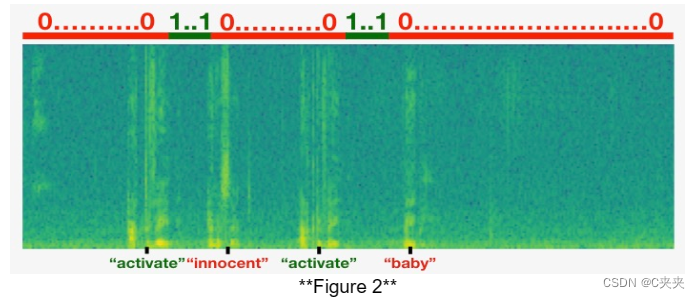
下图说明了标签 y⟨t⟩ ,对于我们插入了“激活”、“无辜”、“激活”、“宝贝”的剪辑。请注意,正面标签“1”仅与正面词相关联。
要实现训练集综合过程,您将使用以下帮助程序函数。所有这些函数都将使用 1ms 的离散化间隔,因此 10 秒的音频被离散化为 10,000 步。
1、get_random_time_segment(segment_ms) 在我们的背景音频中获取一个随机时间段
2、is_overlapping(segment_time, existing_segments) 检查时间段是否与现有段重叠
i3、nsert_audio_clip(background, audio_clip, existing_times) 使用 get_random_time_segment 和 is_overlapping 在我们的背景音频中随机插入一个音频片段
4、insert_ones(y, segment_end_ms) 将 1 插入到标签向量 y 中,在单词 “activate” 之后
函数 get_random_time_segment(segment_ms) 返回一个随机时间段,我们可以在该时间段上插入持续时间为 segment_ms 的音频剪辑。通读代码以确保您了解它正在做什么。
获取持续时间的随机时间段 segment_ms 在 10,000 毫秒的音频剪辑中。
参数:segment_ms -- 音频剪辑的持续时间,单位为毫秒(“毫秒”代表“毫秒”)
返回:segment_time -- (segment_start, segment_end) 的元组,单位为 ms
def get_random_time_segment(segment_ms):
    segment_start = np.random.randint(low=0, high=10000-segment_ms)   # Make sure segment doesn't run past the 10sec background
    segment_end = segment_start + segment_ms - 1

    return (segment_start, segment_end)
接下来,假设您已在段 (1000,1800) 和 (3400,4500) 处插入音频剪辑。即,第一段从步骤 1000 开始,到步骤 1800 结束。现在,如果我们考虑在 (3000,3600) 处插入一个新的音频剪辑,这是否与之前插入的片段之一重叠?在本例中,(3000,3600) 和 (3400,4500) 重叠,因此我们应该决定不在此处插入剪辑。
出于此函数的目的,将 (100,200) 和 (200,250) 定义为重叠,因为它们在时间步长 200 处重叠。但是,(100,199) 和 (200,250) 是不重叠的。
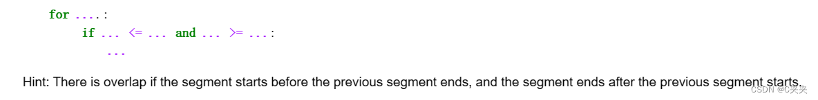
练习:实施 is_overlapping(segment_time, existing_segments) 以检查新时间段是否与之前的任何时间段重叠。您将需要执行 2 个步骤:
1、创建一个“False”标志,如果发现存在重叠,稍后将该标志设置为“True”。
2、循环previous_segments的开始和结束时间。将这些时间与区段的开始和结束时间进行比较。如果存在重叠,请将 (1) 中定义的标志设置为 True。您可以使用:
检查区段的时间是否与现有区段的时间重叠。
参数:
    segment_time -- 新段的 (segment_start, segment_end) 元组
    previous_segments -- 现有段的 (segment_start, segment_end) 元组列表
返回:如果时间段与任何现有段重叠,则为 True,否则为 False
# GRADED FUNCTION: is_overlapping
def is_overlapping(segment_time, previous_segments):
    segment_start, segment_end = segment_time

    # Step 1: Initialize overlap as a "False" flag. (≈ 1 line)
    overlap = False

    # Step 2: loop over the previous_segments start and end times.
    # Compare start/end times and set the flag to True if there is an overlap (≈ 3 lines)
    for previous_start, previous_end in previous_segments:
        if segment_start <= previous_end and segment_end >= previous_start:
            overlap = True

    return overlap

overlap1 = is_overlapping((950, 1430), [(2000, 2550), (260, 949)])
overlap2 = is_overlapping((2305, 2950), [(824, 1532), (1900, 2305), (3424, 3656)])
print("Overlap 1 = ", overlap1)
print("Overlap 2 = ", overlap2)
Overlap 1 False
Overlap 2 True
现在,使用前面的帮助程序函数在随机时间将新的音频剪辑插入到 10 秒背景上,但要确保任何新插入的片段都不会与之前的片段重叠。
练习:实现 insert_audio_clip() 将音频剪辑叠加到背景 10 秒剪辑上。您将需要执行 4 个步骤:
- 获取正确持续时间的随机时间段(以毫秒为单位)。
- 确保该时间段不与之前的任何时间段重叠。如果它重叠,则返回第 1 步并选择新的时间段。
- 将新时间段添加到现有时间段列表中,以便跟踪已插入的所有时间段。
- 使用 pydub 将音频剪辑覆盖在背景上。我们已经为您实现了这一点。
以随机时间步长在背景噪音上插入新的音频片段,确保音频段不与现有段重叠。
参数:
    background -- 10 秒的背景录音。
    audio_clip -- 要插入/覆盖的音频剪辑。
    previous_segments -- 已放置音频段的时间
返回:new_background -- 更新的背景音频
# GRADED FUNCTION: insert_audio_clip
def insert_audio_clip(background, audio_clip, previous_segments):
    # Get the duration of the audio clip in ms
    segment_ms = len(audio_clip)

    # Step 1: Use one of the helper functions to pick a random time segment onto which to insert
    # the new audio clip. (≈ 1 line)
    segment_time = get_random_time_segment(segment_ms)

    # Step 2: Check if the new segment_time overlaps with one of the previous_segments. If so, keep
    # picking new segment_time at random until it doesn't overlap. (≈ 2 lines)
    while is_overlapping(segment_time, previous_segments):
        segment_time = get_random_time_segment(segment_ms)

    # Step 3: Add the new segment_time to the list of previous_segments (≈ 1 line)
    previous_segments.append(segment_time)

    # Step 4: Superpose audio segment and background
    new_background = background.overlay(audio_clip, position = segment_time[0])

    return new_background, segment_time

#上述代码没有问题,结果不一致可能和In[10]说的有关,导致下面到模型前的结果也都不一致
np.random.seed(5)
audio_clip, segment_time = insert_audio_clip(backgrounds[0], activates[0], [(3790, 4400)])
audio_clip.export("insert_test.wav", format="wav")
print("Segment Time: ", segment_time)
IPython.display.Audio("insert_test.wav")
Segment Time (2254, 3169)
# Expected audio
IPython.display.Audio("audio_examples/insert_reference.wav")
最后,实现代码以更新标签 y⟨t⟩,假设您刚刚插入了“激活”。在下面的代码中,y 是一个 (1,1375) 维向量,因为 Ty=1375
如果“激活”在时间步骤t结束,然后设置 y⟨t+1⟩=1以及多达 49 个额外的连续值。但是,请确保不要跑出数组的末尾并尝试更新 y[0][1375],因为有效索引为 y[0][0] 到 y[0][1374],因为 Ty=1375.因此,如果“激活”在步骤 1370 结束,则只会得到 y[0][1371] = y[0][1372] = y[0][1373] = y[0][1374] = 1
练习:实现 insert_ones()。您可以使用 for 循环。(如果你是 python 切片操作的专家,也可以随意使用切片来矢量化它。如果段以 segment_end_ms 结尾(使用 10000 步离散化),将其转换为输出 y 的索引(使用 1375步进离散化),我们将使用以下公式:
segment_end_y = int(segment_end_ms * Ty / 10000.0)
更新标签向量 y。50 个输出步长的标签严格在段结束后应设置为 1。严格来说,我们的意思是 segment_end_y 的标签应该是 0,而应为 50 个 followinf 标签。
参数:
    y -- 形状的 numpy 数组 (1, Ty),训练示例的标签
    segment_end_ms -- 段的结束时间,以毫秒为单位
返回:
    y -- 更新的标签
# GRADED FUNCTION: insert_ones
def insert_ones(y, segment_end_ms):
# duration of the background (in terms of spectrogram time-steps)
segment_end_y = int(segment_end_ms * Ty / 10000.0)
# Add 1 to the correct index in the background label (y)
for i in range(segment_end_y+1, segment_end_y+51):
if i < Ty:
y[0, i] = 1.0
return y
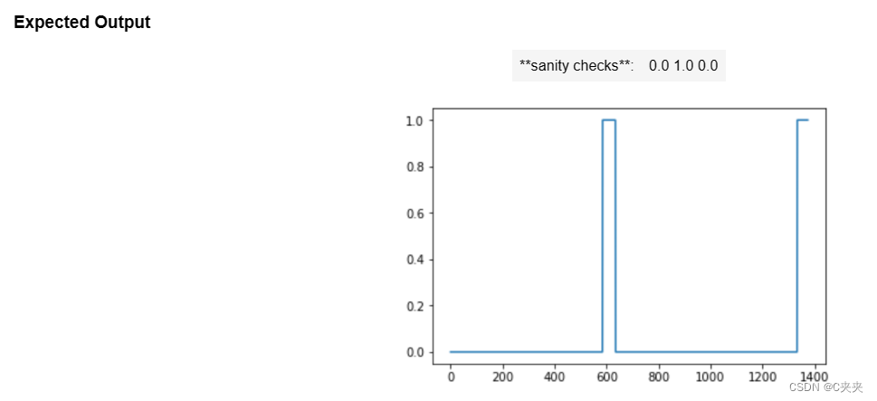
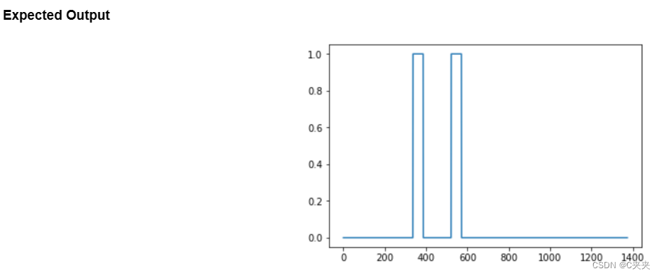
arr1 = insert_ones(np.zeros((1, Ty)), 9700)
plt.plot(insert_ones(arr1, 4251)[0,:])
print("sanity checks:", arr1[0][1333], arr1[0][634], arr1[0][635])
最后,您可以使用 insert_audio_clip 和 insert_ones 创建新的训练示例。
练习:实现 create_training_example()。您将需要执行以下步骤:
- 初始化标签向量 y作为零和形状 (1,Ty) 的 numpy 数组
- 将现有段集初始化为空列表。
- 随机选择 0 到 4 个“激活”音频剪辑,并将它们插入到 10 秒剪辑上。同时在标签向量 y 中的正确位置插入标签
- 随机选择 0 到 2 个负面音频剪辑,并将它们插入 10 秒剪辑中。
创建具有给定背景、激活和负数的训练示例。
参数:
    background -- 10 秒的背景音频录制
    激活 -- 单词“activate”的音频片段列表
    negatives -- 未“激活”的随机单词的音频片段列表
返回:
    x -- 训练示例的频谱图
    y -- 频谱图每个时间步长的标签
# GRADED FUNCTION: create_training_example
def create_training_example(background, activates, negatives):
    # Set the random seed
    np.random.seed(18)

    # Make background quieter
    background = background - 20

    # Step 1: Initialize y (label vector) of zeros (≈ 1 line)

    y = np.zeros((1, Ty))
    # Step 2: Initialize segment times as empty list (≈ 1 line)
    previous_segments = []

    # Select 0-4 random "activate" audio clips from the entire list of "activates" recordings
    number_of_activates = np.random.randint(0, 5)
    random_indices = np.random.randint(len(activates), size=number_of_activates)
    random_activates = [activates[i] for i in random_indices]

    # Step 3: Loop over randomly selected "activate" clips and insert in background
    for random_activate in random_activates:
        # Insert the audio clip on the background
        background, segment_time = insert_audio_clip(background, random_activate, previous_segments)
        # Retrieve segment_start and segment_end from segment_time
        segment_start, segment_end = segment_time
        # Insert labels in "y"
        y = insert_ones(y, segment_end)

    # Select 0-2 random negatives audio recordings from the entire list of "negatives" recordings
    number_of_negatives = np.random.randint(0, 3)
    random_indices = np.random.randint(len(negatives), size=number_of_negatives)
    random_negatives = [negatives[i] for i in random_indices]

    # Step 4: Loop over randomly selected negative clips and insert in background
    for random_negative in random_negatives:

        # Insert the audio clip on the background
        background, _ = background, segment_time = insert_audio_clip(background, random_negative, previous_segments)

    # Standardize the volume of the audio clip
    background = match_target_amplitude(background, -20.0)

    # Export new training example
    file_handle = background.export("train" + ".wav", format="wav")
    print("File (train.wav) was saved in your directory.")

    # Get and plot spectrogram of the new recording (background with superposition of positive and negatives)
    x = graph_spectrogram("train.wav")

    return x, y

x, y = create_training_example(backgrounds[0], activates, negatives)

现在,您可以收听您创建的训练示例,并将其与上面生成的频谱图进行比较。
IPython.display.Audio("train.wav")
Expected Output
IPython.display.Audio("audio_examples/train_reference.wav")
最后,您可以为生成的训练示例绘制关联的标签。
plt.plot(y[0])
4、全套训练集
现在,已经实现了生成单个训练示例所需的代码。我们使用这个过程来生成一个大型训练集。为了节省时间,已经生成了一组训练示例。
# Load preprocessed training examples
X = np.load("./XY_train/X.npy")
Y = np.load("./XY_train/Y.npy")
5、开发集
为了测试我们的模型,我们记录了一组包含 25 个示例的开发。当我们的训练数据被合成时,我们希望使用与真实输入相同的分布来创建一个开发集。因此,我们录制了 25 个 10 秒的音频片段,其中人们说“激活”和其他随机单词,并手工标记它们。这遵循了课程 3 中描述的原则,即我们应该创建尽可能与测试集分布相似的开发集;这就是为什么我们的开发集使用真实音频而不是合成音频的原因。
# Load preprocessed dev set examples
X_dev = np.load("./XY_dev/X_dev.npy")
Y_dev = np.load("./XY_dev/Y_dev.npy")
二、模型
现在,你已经构建了一个数据集,让我们编写和训练一个触发词检测模型!
该模型将使用一维卷积层、GRU 层和密集层。让我们加载允许您在 Keras 中使用这些层的包。这可能需要一分钟才能加载。
from keras.callbacks import ModelCheckpoint
from keras.models import Model, load_model, Sequential
from keras.layers import Dense, Activation, Dropout, Input, Masking, TimeDistributed, LSTM, Conv1D
from keras.layers import GRU, Bidirectional, BatchNormalization, Reshape
from keras.optimizers import Adam
1、建立模型
下面是我们将使用的架构。花一些时间查看模型,看看它是否有意义。
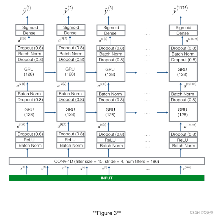
该模型的一个关键步骤是1D卷积步骤(图3底部附近),它输入5511阶跃谱图,输出1375阶跃输出,然后经过多层进一步处理,得到最终的𝑇综=1375步骤的输出。这一层的作用类似于您在课程4中看到的2D卷积,提取低级特征,然后可能生成较小维度的输出。
在计算上,一维转换层也有助于加速模型,因为现在GRU只需要处理1375个时间步长,而不是5511个时间步长。两个GRU层从左到右读取输入序列,然后最终使用密集的+sigmoid层对⟨𝑡⟩进行预测. 因为𝑦如果是二进制值(0或1),我们在最后一层使用sigmoid输出来估计输出为1的可能性,对应于用户刚刚说的“激活”。
注意,我们使用的是单向RNN而不是双向RNN。这对于触发词检测非常重要,因为我们希望能够在触发词被说出后几乎立即检测到它。如果我们使用双向RNN,我们将不得不等待整个10秒的音频被记录下来,然后我们才能判断在音频剪辑的第一秒是否说了“激活”。
实现该模型可分为四个步骤:
- 步骤1:CONV层。使用Conv1D()实现这一点,使用196个过滤器,过滤器大小为15 (kernel_size=15),步长为4。(参见文档。)
- 步骤2:第一个GRU层。要生成GRU层,使用:X = GRU(units = 128, return_sequences = True)(X)
设置return_sequences=True确保所有GRU的隐藏状态都被馈送到下一层。记得在Dropout和BatchNorm图层中遵循这一步骤。 - 步骤3:第二个GRU层。这类似于前面的GRU层(记住使用return_sequences=True),但是有一个额外的dropout层。
- 步骤4:创建一个时间分布的致密层,如下所示:X = timedidistributed (Dense(1, activation = “sigmoid”))(X)
这将创建一个密集层,后面跟着一个s形曲线,因此用于密集层的参数对于每个时间步都是相同的。(参见文档。)
练习:实现模型(),体系结构如图3所示。
在Keras中创建模型图的函数。
参数:input_shape——模型输入数据的形状(使用Keras约定)
返回:model——Keras模型实例
# GRADED FUNCTION: model
def model(input_shape):
    X_input = Input(shape = input_shape)

     # Step 1: CONV layer
    X = Conv1D(196, 15, strides=4)(X_input)             # CONV1D
    X = BatchNormalization()(X)                         # Batch normalization
    X = Activation('relu')(X)                           # ReLu activation
    X = Dropout(0.8)(X)                                 # dropout (use 0.8)

    # Step 2: First GRU Layer
    X = GRU(units = 128, return_sequences = True)(X)    # GRU (use 128 units and return the sequences)
    X = Dropout(0.8)(X)                                 # dropout (use 0.8)
    X = BatchNormalization()(X)                         # Batch normalization

    # Step 3: Second GRU Layer
    X = GRU(units = 128, return_sequences = True)(X)    # GRU (use 128 units and return the sequences)
    X = Dropout(0.8)(X)                                 # dropout (use 0.8)
    X = BatchNormalization()(X)                         # Batch normalization
    X = Dropout(0.8)(X)                                 # dropout (use 0.8)

    # Step 4: Time-distributed dense layer
    X = TimeDistributed(Dense(1, activation = "sigmoid"))(X) # time distributed  (sigmoid)

    model = Model(inputs = X_input, outputs = X)

    return model

model = model(input_shape = (Tx, n_freq))
model.summary()
Total params 522,561
Trainable params 521,657
Non-trainable params 904
网络的输出形状为(None, 1375,1),而输入形状为(None, 5511,101)。Conv1D将频谱图上的步骤数从5511减少到1375。
2、适应模型
触发词检测需要很长时间才能训练。为了节省时间,我们已经使用上面构建的架构在 GPU 上训练了大约 3 个小时的模型,以及大约 4000 个示例的大型训练集。让我们加载模型。
model = load_model('./models/tr_model.h5')
您可以使用 Adam 优化器和二元交叉熵损失进一步训练模型,如下所示。这将很快运行,因为我们只针对一个 epoch 进行训练,并且使用包含 26 个示例的小型训练集。
opt = Adam(lr=0.0001, beta_1=0.9, beta_2=0.999, decay=0.01)
model.compile(loss='binary_crossentropy', optimizer=opt, metrics=["accuracy"])

model.fit(X, Y, batch_size = 5, epochs=1)
3、测试模型
loss, acc = model.evaluate(X_dev, Y_dev)
print("Dev set accuracy = ", acc)
这看起来还不错!然而,对于这项任务来说,准确性并不是一个很好的指标,因为标签严重偏向于0,所以只输出0的神经网络将获得略高于90%的准确率。我们可以定义更有用的指标,例如 F1 分数或精确率/召回率。但是,我们不要在这里打扰它,而只是从经验上看看模型是如何工作的。
在生成的图上,您可以观察预测输出中每个字符的注意力权重值。检查此图并检查网络关注的位置是否对您有意义。
在日期翻译应用程序中,您将观察到,大多数时候注意力有助于预测年份,并且对预测日/月没有太大影响。
三、做出预测
现在,您已经构建了一个用于触发词检测的工作模型,让我们使用它来进行预测。此代码片段通过网络运行音频(保存在 wav 文件中)。
def detect_triggerword(filename):
    plt.subplot(2, 1, 1)

    x = graph_spectrogram(filename)
    # the spectogram outputs (freqs, Tx) and we want (Tx, freqs) to input into the model
    x  = x.swapaxes(0,1)
    x = np.expand_dims(x, axis=0)
    predictions = model.predict(x)

    plt.subplot(2, 1, 2)
    plt.plot(predictions[0,:,0])
    plt.ylabel('probability')
    plt.show()
    return predictions
一旦您估计了在每个输出步骤中检测到单词“激活”的概率,您就可以在概率高于特定阈值时触发“鸣响”声。此外,y⟨t⟩在说“激活”后,连续多个值可能接近 1,但我们只想鸣叫一次。因此,我们最多每 75 个输出步骤插入一次铃声。这将有助于防止我们为单个“activate”实例插入两个提示音。(这起着类似于计算机视觉的非最大抑制的作用。
chime_file = "audio_examples/chime.wav"
def chime_on_activate(filename, predictions, threshold):
    audio_clip = AudioSegment.from_wav(filename)
    chime = AudioSegment.from_wav(chime_file)
    Ty = predictions.shape[1]
    # Step 1: Initialize the number of consecutive output steps to 0
    consecutive_timesteps = 0
    # Step 2: Loop over the output steps in the y
    for i in range(Ty):
        # Step 3: Increment consecutive output steps
        consecutive_timesteps += 1
        # Step 4: If prediction is higher than the threshold and more than 75 consecutive output steps have passed
        if predictions[0,i,0] > threshold and consecutive_timesteps > 75:
            # Step 5: Superpose audio and background using pydub
            audio_clip = audio_clip.overlay(chime, position = ((i / Ty) * audio_clip.duration_seconds)*1000)
            # Step 6: Reset consecutive output steps to 0
            consecutive_timesteps = 0

    audio_clip.export("chime_output.wav", format='wav')
在开发示例上进行测试
IPython.display.Audio("./raw_data/dev/1.wav")
IPython.display.Audio("./raw_data/dev/2.wav")

filename = "./raw_data/dev/1.wav"
prediction = detect_triggerword(filename)
chime_on_activate(filename, prediction, 0.5)
IPython.display.Audio("./chime_output.wav")

filename  = "./raw_data/dev/2.wav"
prediction = detect_triggerword(filename)
chime_on_activate(filename, prediction, 0.5)
IPython.display.Audio("./chime_output.wav")
应该记住的内容:
1、数据合成是为语音问题创建大型训练集的有效方法,特别是触发词检测。
2、在将音频数据传递给 RNN、GRU 或 LSTM 之前,使用频谱图和可选的 1D 卷积层是常见的预处理步骤。
3、端到端的深度学习方法可用于构建非常有效的触发词检测系统。
四、尝试自己例子
在此笔记本的可选且未分级的部分中,您可以在自己的音频剪辑上试用您的模型!
录制一段 10 秒的音频片段,其中您说“激活”一词和其他随机单词,并将其作为 myaudio.wav 上传到 Coursera 中心。请务必将音频作为 wav 文件上传。如果您的音频以不同的格式(例如 mp3)录制,您可以在网上找到用于将其转换为 wav 的免费软件。如果您的录音不是 10 秒,下面的代码将根据需要对其进行修剪或填充,使其为 10 秒。
# Preprocess the audio to the correct format
def preprocess_audio(filename):
    # Trim or pad audio segment to 10000ms
    padding = AudioSegment.silent(duration=10000)
    segment = AudioSegment.from_wav(filename)[:10000]
    segment = padding.overlay(segment)
    # Set frame rate to 44100
    segment = segment.set_frame_rate(44100)
    # Export as wav
    segment.export(filename, format='wav')
将音频文件上传到 Coursera 后,将文件的路径放在下面的变量中。
your_filename = "audio_examples/my_audio.wav"

preprocess_audio(your_filename)
IPython.display.Audio(your_filename) # listen to the audio you uploaded
最后,使用模型预测您在 10 秒音频剪辑中何时说激活,并触发提示音。如果未正确添加哔哔声,请尝试调整chime_threshold。
chime_threshold = 0.5
prediction = detect_triggerword(your_filename)
chime_on_activate(your_filename, prediction, chime_threshold)
IPython.display.Audio("./chime_output.wav")


 3302
3302


 被折叠的 条评论
为什么被折叠?
被折叠的 条评论
为什么被折叠?
 到【灌水乐园】发言


