My First SLAM Implementation EKF-SLAM

最新推荐文章于 2024-06-28 09:41:49 发布

置顶

Snail_Walker

最新推荐文章于 2024-06-28 09:41:49 发布

阅读量2.9k

点赞数 2

分类专栏： RL & DL & SLAM __CMU_ECE_MS_PERIOD__ Autonomous Driving 文章标签： SLAM EKF-SLAM MATLAB

本文链接：https://blog.csdn.net/c602273091/article/details/52695612

版权

本文档详细介绍了作者实现EKF-SLAM的过程，从原理到MATLAB实现，再到结果展示。通过实践，作者强调了EKF-SLAM对SLAM理解的重要性。在原理部分，讨论了状态更新和传感器模型，接着提供了Jacobian矩阵的计算方法。最终，结果显示经过两次递归后，道路路径的估计得到改善。

摘要由CSDN通过智能技术生成

转载请注明出处：http://blog.csdn.net/c602273091/article/details/52695612

ABSTRACT

Learn by doing !

To do it with EKF-SLAM, you can have better comprehensive understanding of SLAM.

PRINCIPLE

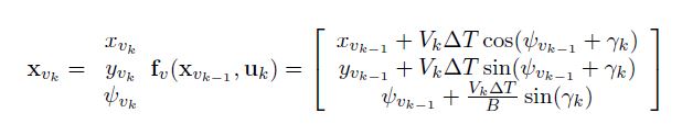
State update by control：（here the control is applied with noise）
这里写图片描述

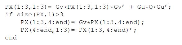
Calculate Predict Covariance:
这里写图片描述

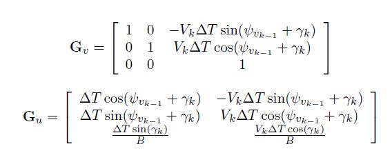
The Jacobian $Gv$ and $Gu$ are calculated by:
这里写图片描述

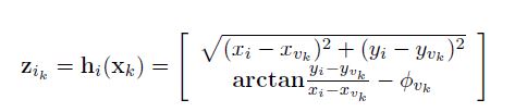
The sensor model is update by:
这里写图片描述

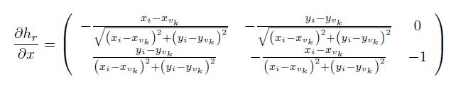
And the Jacobian for robot state is:
这里写图片描述

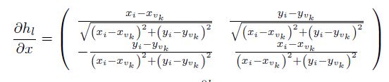
the Jacobian for land mark is:
这里写图片描述

For more details for EKF, search WiKi with EKF.

IMPLEMENTATION

% function my_efk_slam
function my_ekf_2d_slam
    %% load data
    format compact;
    load('example_webmap'); % store in lm, wp
    fig = figure;
    plot(lm(1,:), lm(2,:), 'b*');
    hold on;
    axis equal;
    plot(wp(1,:), wp(2,:), 'g', wp(1,:), wp(2,:), 'g.');
    xlabel('meters'), ylabel('meters');
    set(fig, 'name', 'My 2D EKF-SLAM');

    %% load parameter
    V = 3;% m/s
    MAXG  = 30*pi/180.0;  % maximum steering angles
    RATEG = 20*pi/180.0; % maximum rate of change steering angles
    WHEELBASE   = 4;    % vihecle base
    DT_CONTROLS = 0.025; % seconds between control signals
    sigmaV = 0.3;       % m/s
    sigmaG = (3.0*pi/180); %radians
    Q      = [sigmaV^2 0; 0 sigmaG^2];
    MAX_RANGE = 30.0;   % meters.
    DT_OBSERVE = 8*DT_CONTROLS; % time between observation
    sigmaR = 0.1; 
    sigmaB = (1.0*pi/180);
    R = [sigmaR^2 0; 0 sigmaB^2];
    GATE_REJECT = 4.0;  % maximum dis for creation of new feature.
    GATE_AUGMENT = 25.0; % minimum dis for creation new feature.
    AT_WAYPOINT = 1.0;
    NUMBER_LOOPS = 2; % number of loops through the waypoint list.
    SWITCH_CONTROL_NOISE= 1;