Levenberg–Marquardt算法学习

最新推荐文章于 2021-12-10 22:18:39 发布

taotao1233

最新推荐文章于 2021-12-10 22:18:39 发布

阅读量4.7w

点赞数 33

分类专栏：机器学习文章标签： LevenbergMarquardt 最优化

本文链接：https://blog.csdn.net/jinshengtao/article/details/53310804

版权

机器学习专栏收录该内容

14 篇文章 8 订阅

订阅专栏

本次是对Levenberg–Marquardt的学习总结，是为之后看懂sparse bundle ajdustment打基础。这篇笔记包含如下内容：

回顾高斯牛顿算法，引入LM算法
惩罚因子的计算(迭代步子的计算)
完整的算法流程及代码样例

1. 回顾高斯牛顿，引入LM算法

根据之前的博文： Gauss-Newton算法学习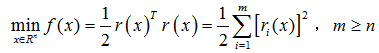

假设我们研究如下形式的非线性最小二乘问题：

r(x)为某个问题的残差residual，是关于x的非线性函数。我们知道高斯牛顿法的迭代公式：

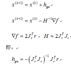
Levenberg–Marquardt算法是对高斯牛顿的改进，在迭代步长上略有不同：

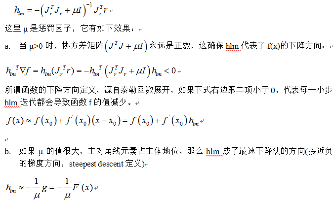
最速下降法对初始点没有特别要求具有整体收敛性，但是相邻两次的搜索方向是相互垂直的，所以收敛并不一定快。总而言之就是：当目标函数的等值线接近于圆(球)时，下降较快；等值线类似于扁长的椭球时，一开始快，后来很慢。This is good if the current iterate is far from the solution.

c. 如果μ的值很小，那么hlm成了高斯牛顿法的方向(适合迭代的最后阶段，非常接近最优解，避免了最速下降的震荡)

由此可见，惩罚因子既下降的方向又影响下降步子的大小。

2. 惩罚因子的计算[迭代步长计算]

我们的目标是求f的最小值，我们希望迭代开始时，惩罚因子μ被设定为较小的值，若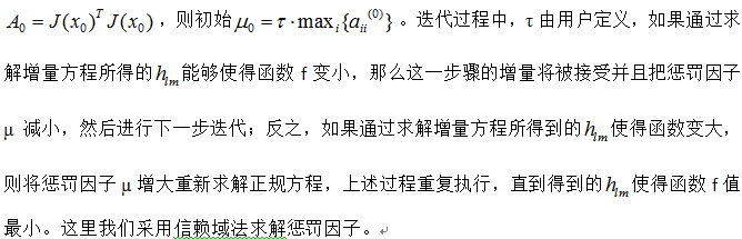

信赖域方法与线搜索技术一样,也是优化算法中的一种保证全局收敛的重要技术. 它们的功能都是在优化算法中求出每次迭代的位移, 从而确定新的迭代点.所不同的是: 线搜索技术是先产生位移方向(亦称为搜索方向), 然后确定位移的长度(亦称为搜索步长)。而信赖域技术则是直接确定位移, 产生新的迭代点。

信赖域方法的基本思想是:首先给定一个所谓的“信赖域半径”作为位移长度的上界，并以当前迭代点为中心以此“上界”为半径确定一个称之为“信赖域”的闭球区域。然后,通过求解这个区域内的“信赖域子问题”(目标函数的二次近似模型) 的最优点来确定“候选位移”。若候选位移能使目标函数值有充分的下降量, 则接受该候选位移作为新的位移,并保持或扩大信赖域半径, 继续新的迭代。否则, 说明二次模型与目标函数的近似度不够理想,需要缩小信赖域半径，再通过求解新的信赖域内的子问题得到新的候选位移。如此重复下去，直到满足迭代终止条件。

现在用信赖域方法解决之前的无约束线性规划：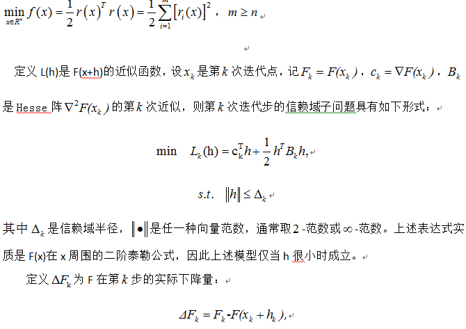

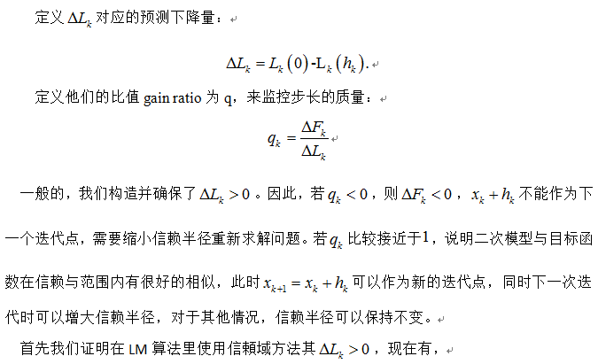
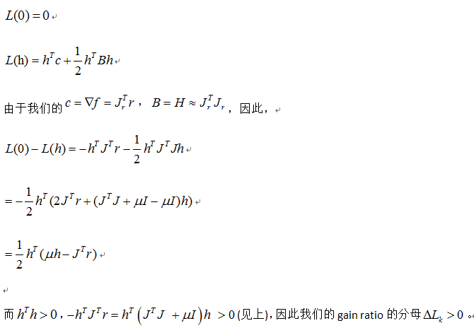
如果q很大，说明L(h)非常接近F(x+h)，我们可以减少惩罚因子μ，以便于下次迭代此时算法更接近高斯牛顿算法。如果q很小或者是负的，说明是poor approximation，我们需要增大惩罚因子，减少步长，此时算法更接近最速下降法。具体来说，

a.当q大于0时，此次迭代有效：

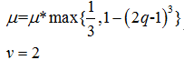
b．当q小于等于0时，此次迭代无效：

3.完整的算法流程及代码距离

LM的算法流程和高斯牛顿几乎一样，只是迭代步长求法利用信赖域法

(1)给定初始点x(0)，允许误差ε>0，置k=0

(2)当f(x^k+1)-f(x^k)小于阈值ε时，算法退出，否则(3)

(3)x^k+1=x^k+hlm，代入f，返回(1)

两个例子还是沿用之前的。

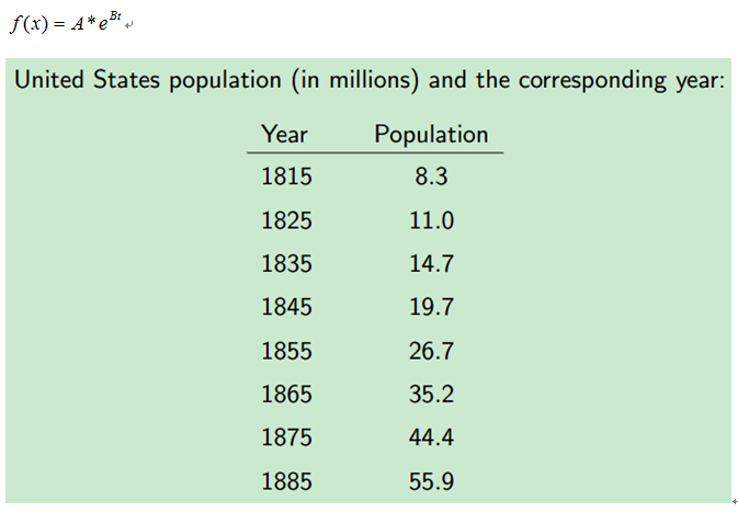
例子1，根据美国1815年至1885年数据，估计人口模型中的参数A和B。如下表所示，已知年份和人口总量，及人口模型方程，求方程中的参数。

// A simple demo of Gauss-Newton algorithm on a user defined function

#include <cstdio>
#include <vector>
#include <opencv2/core/core.hpp>

using namespace std;
using namespace cv;

const double DERIV_STEP = 1e-5;
const int MAX_ITER = 100;


void LM(double(*Func)(const Mat &input, const Mat ¶ms), // function pointer
				 const Mat &inputs, const Mat &outputs, Mat ¶ms);

double Deriv(double(*Func)(const Mat &input, const Mat ¶ms), // function pointer
			 const Mat &input, const Mat ¶ms, int n);

// The user defines their function here
double Func(const Mat &input, const Mat ¶ms);

int main()
{
	// For this demo we're going to try and fit to the function
	// F = A*exp(t*B)
	// There are 2 parameters: A B
	int num_params = 2;

    // Generate random data using these parameters
    int total_data = 8;

    Mat inputs(total_data, 1, CV_64F);
    Mat outputs(total_data, 1, CV_64F);

	//load observation data
    for(int i=0; i < total_data; i++) {
        inputs.at<double>(i,0) = i+1;  //load year
    }
	//load America population
	outputs.at<double>(0,0)= 8.3;
	outputs.at<double>(1,0)= 11.0;
	outputs.at<double>(2,0)= 14.7;
	outputs.at<double>(3,0)= 19.7;
	outputs.at<double>(4,0)= 26.7;
	outputs.at<double>(5,0)= 35.2;
	outputs.at<double>(6,0)= 44.4;
	outputs.at<double>(7,0)= 55.9;

    // Guess the parameters, it should be close to the true value, else it can fail for very sensitive functions!
    Mat params(num_params, 1, CV_64F);

	//init guess
    params.at<double>(0,0) = 6;
	params.at<double>(1,0) = 0.3;

    LM(Func, inputs, outputs, params);

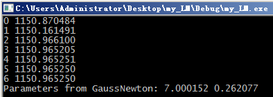
    printf("Parameters from GaussNewton: %lf %lf\n", params.at<double>(0,0), params.at<double>(1,0));

    return 0;
}

double Func(const Mat &input, const Mat ¶ms)
{
	// Assumes input is a single row matrix
	// Assumes params is a column matrix

	double A = params.at<double>(0,0);
	double B = params.at<double>(1,0);

	double x = input.at<double>(0,0);

    return A*exp(x*B);
}

//calc the n-th params' partial derivation ， the params are our  final target
double Deriv(double(*Func)(const Mat &input, const Mat ¶ms), const Mat &input, const Mat ¶ms, int n)
{
	// Assumes input is a single row matrix

	// Returns the derivative of the nth parameter
	Mat params1 = params.clone();
	Mat params2 = params.clone();

	// Use central difference  to get derivative
	params1.at<double>(n,0) -= DERIV_STEP;
	params2.at<double>(n,0) += DERIV_STEP;

	double p1 = Func(input, params1);
	double p2 = Func(input, params2);

	double d = (p2 - p1) / (2*DERIV_STEP);

	return d;
}

void LM(double(*Func)(const Mat &input, const Mat ¶ms),
				 const Mat &inputs, const Mat &outputs, Mat ¶ms)
{
    int m = inputs.rows;
    int n = inputs.cols;
    int num_params = params.rows;

    Mat r(m, 1, CV_64F); // residual matrix
	Mat r_tmp(m, 1, CV_64F);
    Mat Jf(m, num_params, CV_64F); // Jacobian of Func()
    Mat input(1, n, CV_64F); // single row input
	Mat params_tmp = params.clone();

    double last_mse = 0;
	float u = 1, v = 2;
	Mat I = Mat::ones(num_params, num_params, CV_64F);//construct identity matrix
	int i =0;
    for(i=0; i < MAX_ITER; i++) {
        double mse = 0;
		double mse_temp = 0;

        for(int j=0; j < m; j++) {
        	for(int k=0; k < n; k++) {//copy Independent variable vector, the year
        		input.at<double>(0,k) = inputs.at<double>(j,k);
        	}

            r.at<double>(j,0) = outputs.at<double>(j,0) - Func(input, params);//diff between previous estimate and observation population

            mse += r.at<double>(j,0)*r.at<double>(j,0);

            for(int k=0; k < num_params; k++) {
            	Jf.at<double>(j,k) = Deriv(Func, input, params, k);  //construct jacobian matrix
            }
        }

        mse /= m;
        params_tmp = params.clone();
		
		Mat hlm = (Jf.t()*Jf + u*I).inv()*Jf.t()*r;
		params_tmp += hlm; 
		for(int j=0; j < m; j++) {
			r_tmp.at<double>(j,0) = outputs.at<double>(j,0) - Func(input, params_tmp);//diff between current estimate and observation population
			mse_temp += r_tmp.at<double>(j,0)*r_tmp.at<double>(j,0);
		}

		mse_temp /= m;

		Mat q(1,1,CV_64F);
		q = (mse - mse_temp)/(0.5*hlm.t()*(u*hlm-Jf.t()*r));
	    double q_value = q.at<double>(0,0);
		if(q_value>0)
		{
			double s = 1.0/3.0;
			v = 2;
			mse = mse_temp;
			params = params_tmp;
			double temp = 1 - pow(2*q_value-1,3);
			if(s>temp)
			{
				u = u * s;
			}else
			{
				u = u * temp;
			}
		}else
		{
			u = u*v; 
			v = 2*v;
			params = params_tmp;
		}	
		
	
        // The difference in mse is very small, so quit
        if(fabs(mse - last_mse) < 1e-8) {
        	break;
        }

        //printf("%d: mse=%f\n", i, mse);
        printf("%d %lf\n", i, mse);
        last_mse = mse;
    }
}

A=7.0,B=0.26 (初始值，A=6,B=0.3) ，100次迭代到第7次收敛了。和之前差不多，但是LM对于初始的选择是非常敏感的，如果A=6，B=6，则拟合失败！

我调用了matlab的接口跑LM，结果也是一样错误的，图片上可以看到拟合失败

clc;
clear;
a0=[6,6];
options=optimset('Algorithm','Levenberg-Marquardt','Display','iter');
data_1=[1 2 3 4 5 6 7 8];
obs_1=[8.3 11.0 14.7 19.7 26.7 35.2 44.4 55.9];
a=lsqnonlin(@myfun,a0,[],[],options,data_1,obs_1);
plot(data_1,obs_1,'o');
hold on
plot(data_1,a(1)*exp(a(2)*data_1),'b');
plot(data_1,7*exp(a(2)*data_1),'b');
%hold off
a(1)
a(2)




function E = myfun(a, x,y)
%这是一个测试文件用于测试 lsqnonlin
%   Detailed explanation goes here
x=x(:);
y=y(:);
Y=a(1)*exp(a(2)*x);
E=y-Y;
end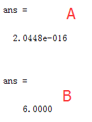

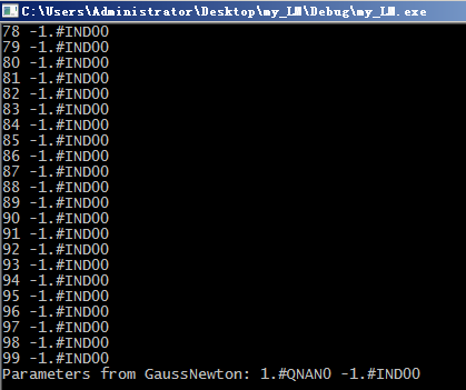
最后一个点拟合失败的，所以函数不对的

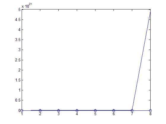
因此虽然莱文博格-马夸特迭代法能够自适应的在高斯牛顿和最速下降法之间调整，既可保证在收敛较慢时迭代过程总是下降的，又可保证迭代过程在解的邻域内迅速收敛。但是，LM对于初始点选择还是比较敏感的！

例子2：我想要拟合如下模型，

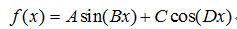
由于缺乏观测量，就自导自演，假设4个参数已知A=5,B=1,C=10,D=2，构造100个随机数作为x的观测值，计算相应的函数观测值。然后，利用这些观测值，反推4个参数。

// A simple demo of Gauss-Newton algorithm on a user defined function

#include <cstdio>
#include <vector>
#include <opencv2/core/core.hpp>

using namespace std;
using namespace cv;

const double DERIV_STEP = 1e-5;
const int MAX_ITER = 100;


void LM(double(*Func)(const Mat &input, const Mat ¶ms), // function pointer
				 const Mat &inputs, const Mat &outputs, Mat ¶ms);

double Deriv(double(*Func)(const Mat &input, const Mat ¶ms), // function pointer
			 const Mat &input, const Mat ¶ms, int n);

// The user defines their function here
double Func(const Mat &input, const Mat ¶ms);

int main()
{
	// For this demo we're going to try and fit to the function
	// F = A*sin(Bx) + C*cos(Dx)
	// There are 4 parameters: A, B, C, D
	int num_params = 4;

    // Generate random data using these parameters
    int total_data = 100;

    double A = 5;
    double B = 1;
    double C = 10;
    double D = 2;

    Mat inputs(total_data, 1, CV_64F);
    Mat outputs(total_data, 1, CV_64F);

    for(int i=0; i < total_data; i++) {
        double x = -10.0 + 20.0* rand() / (1.0 + RAND_MAX); // random between [-10 and 10]
        double y = A*sin(B*x) + C*cos(D*x);

        // Add some noise
       // y += -1.0 + 2.0*rand() / (1.0 + RAND_MAX);

        inputs.at<double>(i,0) = x;
        outputs.at<double>(i,0) = y;
    }

    // Guess the parameters, it should be close to the true value, else it can fail for very sensitive functions!
    Mat params(num_params, 1, CV_64F);

    params.at<double>(0,0) = 1;
    params.at<double>(1,0) = 1;
    params.at<double>(2,0) = 8; // changing to 1 will cause it not to find the solution, too far away
    params.at<double>(3,0) = 1;

    LM(Func, inputs, outputs, params);

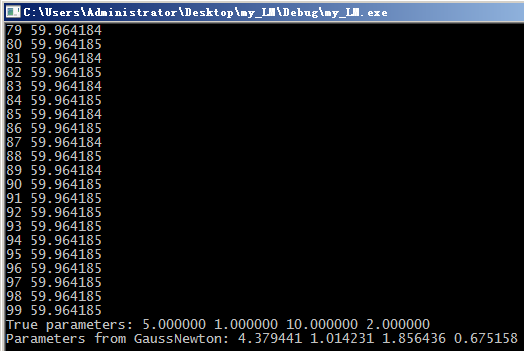
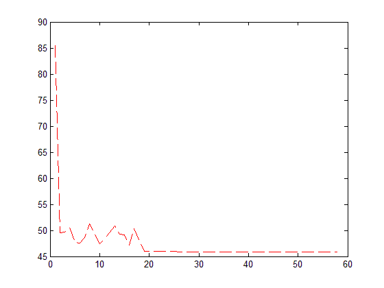
    printf("True parameters: %f %f %f %f\n", A, B, C, D);
    printf("Parameters from GaussNewton: %f %f %f %f\n", params.at<double>(0,0), params.at<double>(1,0),
    													params.at<double>(2,0), params.at<double>(3,0));

    return 0;
}

double Func(const Mat &input, const Mat ¶ms)
{
	// Assumes input is a single row matrix
	// Assumes params is a column matrix

	double A = params.at<double>(0,0);
	double B = params.at<double>(1,0);
	double C = params.at<double>(2,0);
	double D = params.at<double>(3,0);

	double x = input.at<double>(0,0);

    return A*sin(B*x) + C*cos(D*x);
}

//calc the n-th params' partial derivation ， the params are our  final target
double Deriv(double(*Func)(const Mat &input, const Mat ¶ms), const Mat &input, const Mat ¶ms, int n)
{
	// Assumes input is a single row matrix

	// Returns the derivative of the nth parameter
	Mat params1 = params.clone();
	Mat params2 = params.clone();

	// Use central difference  to get derivative
	params1.at<double>(n,0) -= DERIV_STEP;
	params2.at<double>(n,0) += DERIV_STEP;

	double p1 = Func(input, params1);
	double p2 = Func(input, params2);

	double d = (p2 - p1) / (2*DERIV_STEP);

	return d;
}

void LM(double(*Func)(const Mat &input, const Mat ¶ms),
				 const Mat &inputs, const Mat &outputs, Mat ¶ms)
{
    int m = inputs.rows;
    int n = inputs.cols;
    int num_params = params.rows;

    Mat r(m, 1, CV_64F); // residual matrix
	Mat r_tmp(m, 1, CV_64F);
    Mat Jf(m, num_params, CV_64F); // Jacobian of Func()
    Mat input(1, n, CV_64F); // single row input
	Mat params_tmp = params.clone();

    double last_mse = 0;
	float u = 1, v = 2;
	Mat I = Mat::ones(num_params, num_params, CV_64F);//construct identity matrix
	int i =0;
    for(i=0; i < MAX_ITER; i++) {
        double mse = 0;
		double mse_temp = 0;

        for(int j=0; j < m; j++) {
        	for(int k=0; k < n; k++) {//copy Independent variable vector, the year
        		input.at<double>(0,k) = inputs.at<double>(j,k);
        	}

            r.at<double>(j,0) = outputs.at<double>(j,0) - Func(input, params);//diff between estimate and observation population

            mse += r.at<double>(j,0)*r.at<double>(j,0);

            for(int k=0; k < num_params; k++) {
            	Jf.at<double>(j,k) = Deriv(Func, input, params, k);  //construct jacobian matrix
            }
        }

        mse /= m;
        params_tmp = params.clone();
		
		Mat hlm = (Jf.t()*Jf + u*I).inv()*Jf.t()*r;
		params_tmp += hlm; 
		for(int j=0; j < m; j++) {
			r_tmp.at<double>(j,0) = outputs.at<double>(j,0) - Func(input, params_tmp);//diff between estimate and observation population
			mse_temp += r_tmp.at<double>(j,0)*r_tmp.at<double>(j,0);
		}

		mse_temp /= m;

		Mat q(1,1,CV_64F);
		q = (mse - mse_temp)/(0.5*hlm.t()*(u*hlm-Jf.t()*r));
	    double q_value = q.at<double>(0,0);
		if(q_value>0)
		{
			double s = 1.0/3.0;
			v = 2;
			mse = mse_temp;
			params = params_tmp;
			double temp = 1 - pow(2*q_value-1,3);
			if(s>temp)
			{
				u = u * s;
			}else
			{
				u = u * temp;
			}
		}else
		{
			u = u*v; 
			v = 2*v;
			params = params_tmp;
		}	
		
	
        // The difference in mse is very small, so quit
        if(fabs(mse - last_mse) < 1e-8) {
        	break;
        }

        //printf("%d: mse=%f\n", i, mse);
        printf("%d %lf\n", i, mse);
        last_mse = mse;
    }
}

我们看到迭代了100次，结果几何和高斯牛顿算出来是一样的。我们绘制LM和高斯牛顿的残差函数收敛过程，发现 LM一直是总体下降的，没有太多反复。

高斯牛顿：

LM：

taotao1233

关注

33
点赞
踩
258

收藏

觉得还不错? 一键收藏
5
评论
Levenberg–Marquardt算法学习

本次是对Levenberg–Marquardt的学习总结，是为之后看懂sparse bundle ajdustment打基础。这篇笔记包含如下内容：回顾高斯牛顿算法，引入LM算法惩罚因子的计算(迭代步子的计算)完整的算法流程及代码样例1. 回顾高斯牛顿，引入LM算法根据之前的博文：Gauss-Newton算法学习假设我们研究如下形式的非线性最小二乘问题： r(x)为某个问题的残差
复制链接

扫一扫