


Gauss-Newton算法是解决非线性最优问题的常见算法之一,最近研读开源项目代码,又碰到了,索性深入看下。本次讲解内容如下:
- 基本数学名词识记
- 牛顿法推导、算法步骤、计算实例
- 高斯牛顿法推导(如何从牛顿法派生)、算法步骤、编程实例
- 高斯牛顿法优劣总结
一、基本概念定义
1.非线性方程定义及最优化方法简述
指因变量与自变量之间的关系不是线性的关系,比如平方关系、对数关系、指数关系、三角函数关系等等。对于此类方程,求解n元实函数f在整个n维向量空间Rn上的最优值点往往很难得到精确解,经常需要求近似解问题。
求解该最优化问题的方法大多是逐次一维搜索的迭代算法,基本思想是在一个近似点处选定一个有利于搜索方向,沿这个方向进行一维搜索,得到新的近似点。如此反复迭代,知道满足预定的精度要求为止。根据搜索方向的取法不同,这类迭代算法可分为两类:
解析法:需要用目标函数的到函数,
梯度法:又称最速下降法,是早期的解析法,收敛速度较慢
牛顿法:收敛速度快,但不稳定,计算也较困难。高斯牛顿法基于其改进,但目标作用不同
共轭梯度法:收敛较快,效果好
变尺度法:效率较高,常用DFP法(Davidon Fletcher Powell)
直接法:不涉及导数,只用到函数值。有交替方向法(又称坐标轮换法)、模式搜索法、旋转方向法、鲍威尔共轭方向法和单纯形加速法等。
2.非线性最小二乘问题
非线性最小二乘问题来自于非线性回归,即通过观察自变量和因变量数据,求非线性目标函数的系数参数,使得函数模型与观测量尽量相似。
高斯牛顿法解决非线性最小二乘问题的最基本方法,并且它只能处理二次函数。(使用时必须将目标函数转化为二次的)
Unlike Newton'smethod, the Gauss–Newton algorithm can only be used to minimize a sum ofsquared function values
3.基本数学表达
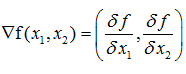
a.梯度gradient,由多元函数的各个偏导数组成的向量
以二元函数为例,其梯度为:
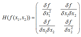
b.黑森矩阵Hessian matrix,由多元函数的二阶偏导数组成的方阵,描述函数的局部曲率,以二元函数为例,
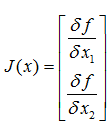
c.雅可比矩阵 Jacobian matrix,是多元函数一阶偏导数以一定方式排列成的矩阵,体现了一个可微方程与给出点的最优线性逼近。以二元函数为例,
如果扩展多维的话F: Rn-> Rm,则雅可比矩阵是一个m行n列的矩阵:
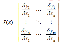
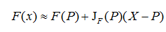
雅可比矩阵作用,如果P是Rn中的一点,F在P点可微分,那么在这一点的导数由JF(P)给出,在此情况下,由F(P)描述的线性算子即接近点P的F的最优线性逼近:
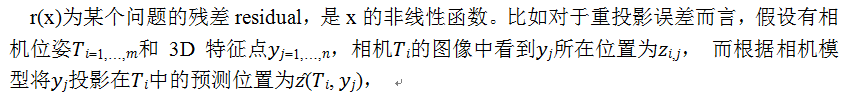
d.残差 residual,表示实际观测值与估计值(拟合值)之间的差
二、牛顿法
牛顿法的基本思想是采用多项式函数来逼近给定的函数值,然后求出极小点的估计值,重复操作,直到达到一定精度为止。
1.考虑如下一维无约束的极小化问题:
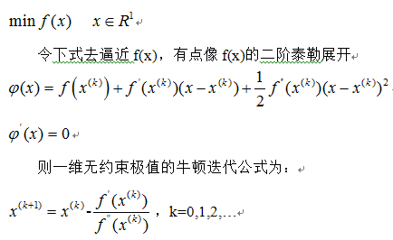
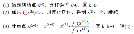
因此,一维牛顿法的计算步骤如下:
需要注意的是,牛顿法在求极值的时候,如果初始点选取不好,则可能不收敛于极小点
2.下面给出多维无约束极值的情形:
若非线性目标函数f(x)具有二阶连续偏导,在x(k)为其极小点的某一近似,在这一点取f(x)的二阶泰勒展开,即:
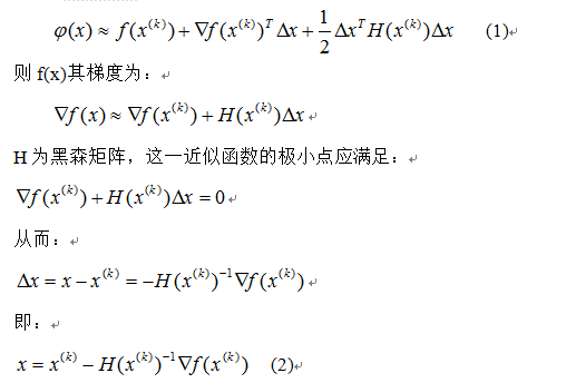
如果f(x)是二次函数,则其黑森矩阵H为常数,式(1)是精确的(等于号),在这种情况下,从任意一点处罚,用式(2)只要一步可求出f(x)的极小点(假设黑森矩阵正定,所有特征值大于0)
如果f(x)不是二次函数,式(1)仅是一个近似表达式,此时,按式(2)求得的极小点,只是f(x)的近似极小点。在这种情况下,常按照下面选取搜索方向:
牛顿法收敛的速度很快,当f(x)的二阶导数及其黑森矩阵的逆矩阵便于计算时,这一方法非常有效。【但通常黑森矩阵很不好求】
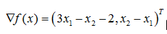
3.下面给出一个实际计算例子。
例:试用牛顿法求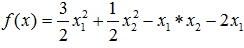
解:
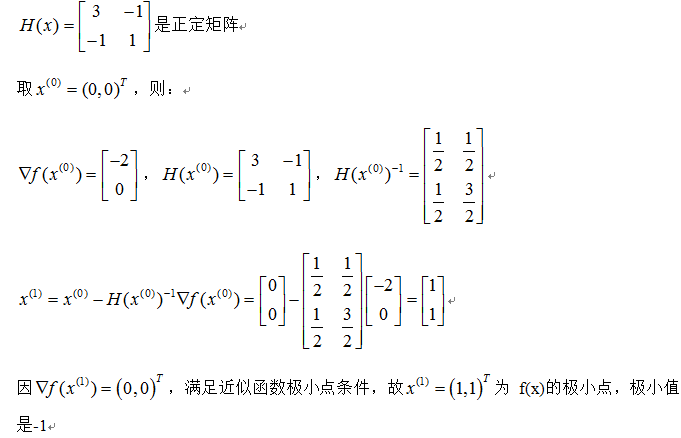
【f(x)是二次函数,H矩阵为常数,只要任意点出发,只要一步即可求出极小点】
三、牛顿高斯法
1. gauss-newton是如何由上述派生的
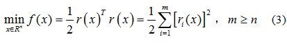
有时候为了拟合数据,比如根据重投影误差求相机位姿(R,T为方程系数),常常将求解模型转化为非线性最小二乘问题。高斯牛顿法正是用于解决非线性最小二乘问题,达到数据拟合、参数估计和函数估计的目的。
假设我们研究如下形式的非线性最小二乘问题:
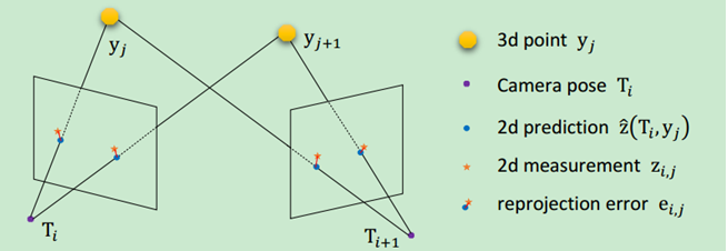
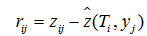
这两个位置间残差(重投影误差):
如果有大量观测点(多维),我们可以通过选择合理的T使得残差的平方和最小求得两个相机之间的位姿。机器视觉这块暂时不扩展,接着说怎么求非线性最小二乘问题。
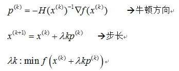
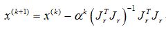
若用牛顿法求式3,则牛顿迭代公式为:
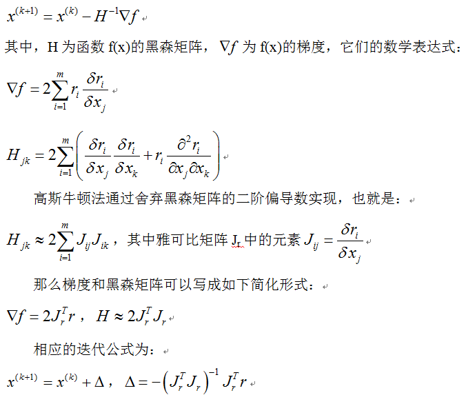
看到这里大家都明白高斯牛顿和牛顿法的差异了吧,就在这迭代项上。经典高斯牛顿算法迭代步长λ为1.
那回过头来,高斯牛顿法里为啥要舍弃黑森矩阵的二阶偏导数呢?主要问题是因为牛顿法中Hessian矩阵中的二阶信息项通常难以计算或者花费的工作量很大,而利用整个H的割线近似也不可取,因为在计算梯度 时已经得到J(x),这样H中的一阶信息项J
TJ几乎是现成的。鉴于此,为了简化计算,获得有效算法,我们可用一阶导数信息逼近二阶信息项。
注意这么干的前提是,残差r接近于零或者接近线性函数从而
时已经得到J(x),这样H中的一阶信息项J
TJ几乎是现成的。鉴于此,为了简化计算,获得有效算法,我们可用一阶导数信息逼近二阶信息项。
注意这么干的前提是,残差r接近于零或者接近线性函数从而 接近与零时,二阶信息项才可以忽略。通常称为“小残量问题”,否则高斯牛顿法不收敛。
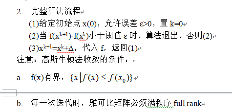
3. 举例
接下来的代码里并没有保证算法收敛的机制,在例子2的自嗨中可以看到劣势。关于自变量维数,代码可以支持多元,但两个例子都是一维的,比如例子1中只有年份t,其实可以增加其他因素的,不必在意。
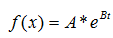
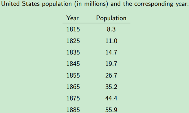
例子1,根据美国1815年至1885年数据,估计人口模型中的参数A和B。如下表所示,已知年份和人口总量,及人口模型方程,求方程中的参数。
// A simple demo of Gauss-Newton algorithm on a user defined function

#include <cstdio>
#include <vector>
#include <opencv2/core/core.hpp>

using namespace std;
using namespace cv;

const double DERIV_STEP = 1e-5;
const int MAX_ITER = 100;


void GaussNewton(double(*Func)(const Mat &input, const Mat ¶ms), // function pointer
				 const Mat &inputs, const Mat &outputs, Mat ¶ms);

double Deriv(double(*Func)(const Mat &input, const Mat ¶ms), // function pointer
			 const Mat &input, const Mat ¶ms, int n);

// The user defines their function here
double Func(const Mat &input, const Mat ¶ms);

int main()
{
	// For this demo we're going to try and fit to the function
	// F = A*exp(t*B)
	// There are 2 parameters: A B
	int num_params = 2;

    // Generate random data using these parameters
    int total_data = 8;

    Mat inputs(total_data, 1, CV_64F);
    Mat outputs(total_data, 1, CV_64F);

	//load observation data
    for(int i=0; i < total_data; i++) {
        inputs.at<double>(i,0) = i+1;  //load year
    }
	//load America population
	outputs.at<double>(0,0)= 8.3;
	outputs.at<double>(1,0)= 11.0;
	outputs.at<double>(2,0)= 14.7;
	outputs.at<double>(3,0)= 19.7;
	outputs.at<double>(4,0)= 26.7;
	outputs.at<double>(5,0)= 35.2;
	outputs.at<double>(6,0)= 44.4;
	outputs.at<double>(7,0)= 55.9;

    // Guess the parameters, it should be close to the true value, else it can fail for very sensitive functions!
    Mat params(num_params, 1, CV_64F);

	//init guess
    params.at<double>(0,0) = 6;
	params.at<double>(1,0) = 0.3;

    GaussNewton(Func, inputs, outputs, params);

    printf("Parameters from GaussNewton: %f %f\n", params.at<double>(0,0), params.at<double>(1,0));

    return 0;
}

double Func(const Mat &input, const Mat ¶ms)
{
	// Assumes input is a single row matrix
	// Assumes params is a column matrix

	double A = params.at<double>(0,0);
	double B = params.at<double>(1,0);

	double x = input.at<double>(0,0);

    return A*exp(x*B);
}

//calc the n-th params' partial derivation , the params are our  final target
double Deriv(double(*Func)(const Mat &input, const Mat ¶ms), const Mat &input, const Mat ¶ms, int n)
{
	// Assumes input is a single row matrix

	// Returns the derivative of the nth parameter
	Mat params1 = params.clone();
	Mat params2 = params.clone();

	// Use central difference  to get derivative
	params1.at<double>(n,0) -= DERIV_STEP;
	params2.at<double>(n,0) += DERIV_STEP;

	double p1 = Func(input, params1);
	double p2 = Func(input, params2);

	double d = (p2 - p1) / (2*DERIV_STEP);

	return d;
}

void GaussNewton(double(*Func)(const Mat &input, const Mat ¶ms),
				 const Mat &inputs, const Mat &outputs, Mat ¶ms)
{
    int m = inputs.rows;
    int n = inputs.cols;
    int num_params = params.rows;

    Mat r(m, 1, CV_64F); // residual matrix
    Mat Jf(m, num_params, CV_64F); // Jacobian of Func()
    Mat input(1, n, CV_64F); // single row input

    double last_mse = 0;

    for(int i=0; i < MAX_ITER; i++) {
        double mse = 0;

        for(int j=0; j < m; j++) {
        	for(int k=0; k < n; k++) {//copy Independent variable vector, the year
        		input.at<double>(0,k) = inputs.at<double>(j,k);
        	}

            r.at<double>(j,0) = outputs.at<double>(j,0) - Func(input, params);//diff between estimate and observation population

            mse += r.at<double>(j,0)*r.at<double>(j,0);

            for(int k=0; k < num_params; k++) {
            	Jf.at<double>(j,k) = Deriv(Func, input, params, k);
            }
        }

        mse /= m;

        // The difference in mse is very small, so quit
        if(fabs(mse - last_mse) < 1e-8) {
        	break;
        }

        Mat delta = ((Jf.t()*Jf)).inv() * Jf.t()*r;
        params += delta;

        //printf("%d: mse=%f\n", i, mse);
        printf("%d %f\n", i, mse);

        last_mse = mse;
    }
}
运行结果:
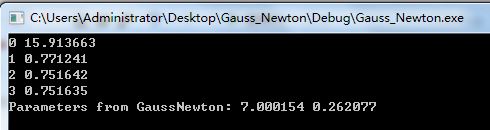
A=7.0,B=0.26 (初始值,A=6,B=0.3),100次迭代到第4次就收敛了。
若初始值A=1,B=1,则要迭代14次收敛。
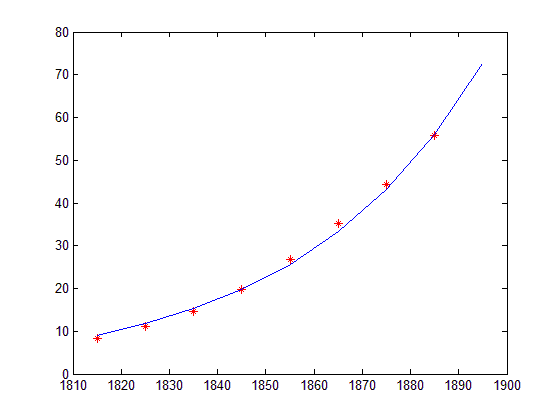
下图为根据上面得到的A、B系数,利用matlab拟合的人口模型曲线
例子2:我想要拟合如下模型,
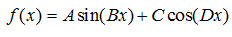
由于缺乏观测量,就自导自演,假设4个参数已知A=5,B=1,C=10,D=2,构造100个随机数作为x的观测值,计算相应的函数观测值。然后,利用这些观测值,反推4个参数。
// A simple demo of Gauss-Newton algorithm on a user defined function

#include <cstdio>
#include <vector>
#include <opencv2/core/core.hpp>

using namespace std;
using namespace cv;

const double DERIV_STEP = 1e-5;
const int MAX_ITER = 100;


void GaussNewton(double(*Func)(const Mat &input, const Mat ¶ms), // function pointer
				 const Mat &inputs, const Mat &outputs, Mat ¶ms);

double Deriv(double(*Func)(const Mat &input, const Mat ¶ms), // function pointer
			 const Mat &input, const Mat ¶ms, int n);

// The user defines their function here
double Func(const Mat &input, const Mat ¶ms);

int main()
{
	// For this demo we're going to try and fit to the function
	// F = A*sin(Bx) + C*cos(Dx)
	// There are 4 parameters: A, B, C, D
	int num_params = 4;

    // Generate random data using these parameters
    int total_data = 100;

    double A = 5;
    double B = 1;
    double C = 10;
    double D = 2;

    Mat inputs(total_data, 1, CV_64F);
    Mat outputs(total_data, 1, CV_64F);

    for(int i=0; i < total_data; i++) {
        double x = -10.0 + 20.0* rand() / (1.0 + RAND_MAX); // random between [-10 and 10]
        double y = A*sin(B*x) + C*cos(D*x);

        // Add some noise
       // y += -1.0 + 2.0*rand() / (1.0 + RAND_MAX);

        inputs.at<double>(i,0) = x;
        outputs.at<double>(i,0) = y;
    }

    // Guess the parameters, it should be close to the true value, else it can fail for very sensitive functions!
    Mat params(num_params, 1, CV_64F);

    params.at<double>(0,0) = 1;
    params.at<double>(1,0) = 1;
    params.at<double>(2,0) = 8; // changing to 1 will cause it not to find the solution, too far away
    params.at<double>(3,0) = 1;

    GaussNewton(Func, inputs, outputs, params);

    printf("True parameters: %f %f %f %f\n", A, B, C, D);
    printf("Parameters from GaussNewton: %f %f %f %f\n", params.at<double>(0,0), params.at<double>(1,0),
    													params.at<double>(2,0), params.at<double>(3,0));

    return 0;
}

double Func(const Mat &input, const Mat ¶ms)
{
	// Assumes input is a single row matrix
	// Assumes params is a column matrix

	double A = params.at<double>(0,0);
	double B = params.at<double>(1,0);
	double C = params.at<double>(2,0);
	double D = params.at<double>(3,0);

	double x = input.at<double>(0,0);

    return A*sin(B*x) + C*cos(D*x);
}

double Deriv(double(*Func)(const Mat &input, const Mat ¶ms), const Mat &input, const Mat ¶ms, int n)
{
	// Assumes input is a single row matrix

	// Returns the derivative of the nth parameter
	Mat params1 = params.clone();
	Mat params2 = params.clone();

	// Use central difference  to get derivative
	params1.at<double>(n,0) -= DERIV_STEP;
	params2.at<double>(n,0) += DERIV_STEP;

	double p1 = Func(input, params1);
	double p2 = Func(input, params2);

	double d = (p2 - p1) / (2*DERIV_STEP);

	return d;
}

void GaussNewton(double(*Func)(const Mat &input, const Mat ¶ms),
				 const Mat &inputs, const Mat &outputs, Mat ¶ms)
{
    int m = inputs.rows;
    int n = inputs.cols;
    int num_params = params.rows;

    Mat r(m, 1, CV_64F); // residual matrix
    Mat Jf(m, num_params, CV_64F); // Jacobian of Func()
    Mat input(1, n, CV_64F); // single row input

    double last_mse = 0;

    for(int i=0; i < MAX_ITER; i++) {
        double mse = 0;

        for(int j=0; j < m; j++) {
        	for(int k=0; k < n; k++) {
        		input.at<double>(0,k) = inputs.at<double>(j,k);
        	}

            r.at<double>(j,0) = outputs.at<double>(j,0) - Func(input, params);

            mse += r.at<double>(j,0)*r.at<double>(j,0);

            for(int k=0; k < num_params; k++) {
            	Jf.at<double>(j,k) = Deriv(Func, input, params, k);
            }
        }

        mse /= m;

        // The difference in mse is very small, so quit
        if(fabs(mse - last_mse) < 1e-8) {
        	break;
        }

        Mat delta = ((Jf.t()*Jf)).inv() * Jf.t()*r;
        params += delta;

        //printf("%d: mse=%f\n", i, mse);
        printf("%f\n",mse);

        last_mse = mse;
    }
}
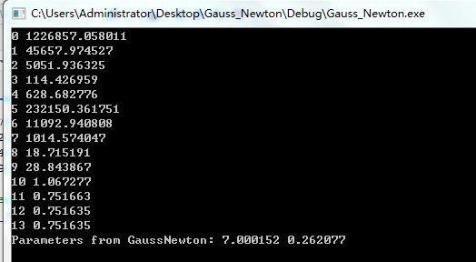
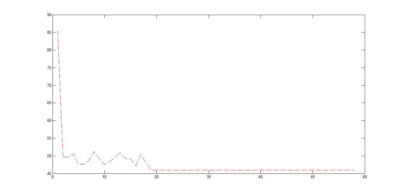
运行结果,得到的参数并不够理想,50次后收敛了
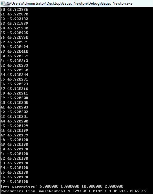
下图中,每次迭代残差并没有持续减少,有反复
4.优缺点分析
优点:
对于零残量问题,即r=0,有局部二阶收敛速度
对于小残量问题,即r较小或接近线性,有快的局部收敛速度
对于线性最小二乘问题,一步达到极小点
缺点:
对于不是很严重的大残量问题,有较慢的局部收敛速度
对于残量很大的问题或r的非线性程度很大的问题,不收敛
不一定总体收敛
如果J不满秩,则方法无定义
对于它的缺点,我们通过增加线性搜索策略,保证目标函数每一步下降,对于几乎所有非线性最小二乘问题,它都具有局部收敛性及总体收敛,即所谓的阻尼高斯牛顿法。
其中,ak为一维搜索因子


 2462
2462

 被折叠的 条评论
为什么被折叠?
被折叠的 条评论
为什么被折叠?
 到【灌水乐园】发言


