【NeurIPS 2021】Autoformer、源码论文对照

dearr__

已于 2025-03-18 15:32:07 修改

阅读量699

点赞数 26

分类专栏：时间序列读文献文章标签：笔记

于 2025-03-18 12:53:59 首次发布

本文链接：https://blog.csdn.net/2301_77549977/article/details/146335872

版权

读文献同时被 2 个专栏收录

24 篇文章

订阅专栏

时间序列

14 篇文章

订阅专栏

吴海旭，徐介晖，王建民，龙明盛

摘要

Extending the forecasting time is a critical demand for real applications, such as extreme weather early warning and long-term energy consumption planning.

This paper studies the long-term forecasting problem of time series.

Prior Transformerbased models adopt various self-attention mechanisms to discover the long-range dependencies.

将预测时间延长是实际应用中的一个关键需求，例如极端天气预警和长期能源消耗规划。本文研究了时间序列的长期预测问题。

此前基于Transformer的模型采用了各种自注意力机制来发现长距离依赖关系。

However, intricate temporal patterns of the long-term future prohibit the model from finding reliable dependencies.

Also, Transformers have to adopt the sparse versions of point-wise self-attentions for long series efficiency, resulting in the information utilization bottleneck.

Going beyond Transformers, we design Autoformer as a novel decomposition architecture with an Auto-Correlation mechanism.

We break with the pre-processing convention of series decomposition and renovate it as a basic inner block of deep models.

然而，长期未来的复杂时间模式阻碍了模型发现可靠的依赖关系。此外，为了提高长序列的效率，Transformer不得不采用稀疏版本的逐点自注意力机制，这导致了信息利用的瓶颈。超越Transformer的范畴，我们设计了Autoformer作为一种具有自相关机制的新型分解架构。我们打破了序列分解的预处理传统，并将其改造为深度模型的基本内部模块。

This design empowers Autoformer with progressive decomposition capacities for complex time series.

Further, inspired by the stochastic process theory, we design the Auto-Correlation mechanism based on the series periodicity, which conducts the dependencies discovery and representation aggregation at the sub-series level.

Auto-Correlation outperforms self-attention in both efficiency and accuracy. In long-term forecasting, Autoformer yields stateof-the-art accuracy, with a 38% relative improvement on six benchmarks, covering five practical applications: energy, traffic, economics, weather and disease. Code is available at this repository: https://github.com/thuml/Autoformer.

这种设计使Autoformer具备了对复杂时间序列进行逐步分解的能力。此外，受随机过程理论的启发，我们基于时间序列的周期性设计了自相关机制（Auto-Correlation mechanism），该机制能够在子序列级别发现依赖关系并聚合表示。

与自注意力机制相比，自相关机制在效率和准确性方面均表现出色。在长期预测方面，Autoformer达到了最先进的精度水平，在涵盖能源、交通、经济、天气和疾病五个实际应用领域的六个基准测试中，相对改进幅度达到了38%。代码已开源，可在以下仓库中获取：<https://github.com/thuml/Autoformer>。

引入

Time series forecasting has been widely used in energy consumption, traffic and economics planning, weather and disease propagation forecasting.

In these real-world applications, one pressing demand is to extend the forecast time into the far future, which is quite meaningful for the long-term planning and early warning.

Thus, in this paper, we study the long-term forecasting problem of time series, characterizing itself by the large length of predicted time series. Recent deep forecasting models [41, 17, 20, 28, 23, 29, 19, 35] have achieved great progress, especially the Transformer-based models.

Benefiting from the self-attention mechanism, Transformers obtain great advantage in modeling long-term dependencies for sequential data, which enables more powerful big models [7, 11].

时间序列预测已在能源消耗、交通规划、经济规划、天气预测以及疾病传播预测中得到了广泛应用。在这些实际应用中，一个迫切的需求是将预测时间延长至更远的未来，这对于长期规划和早期预警具有重要意义。因此，本文研究了时间序列的长期预测问题，其特点是预测时间序列的长度较大。近年来，深度预测模型（如文献[41, 17, 20, 28, 23, 29, 19, 35]）取得了显著进展，尤其是基于Transformer的模型。得益于自注意力机制，Transformer在建模序列数据的长期依赖关系方面具有巨大优势，这使得更强大的大型模型得以实现[7, 11]。

However, the forecasting task is extremely challenging under the long-term setting.

First, it is unreliable to discover the temporal dependencies directly from the long-term time series because the dependencies can be obscured by entangled temporal patterns.

Second, canonical Transformers with self-attention mechanisms are computationally prohibitive for long-term forecasting because of the quadratic complexity of sequence length.

Previous Transformer-based forecasting models [41, 17, 20] mainly focus on improving self-attention to a sparse version.

While performance is significantly improved, these models still utilize the point-wise representation aggregation.

Thus, in the process of efficiency improvement, they will sacrifice the information utilization because of the sparse point-wise connections, resulting in a bottleneck for long-term forecasting of time series.

然而，在长期预测的设定下，预测任务极具挑战性。

首先，直接从长期时间序列中发现时间依赖关系是不可靠的，因为这些依赖关系可能会被复杂交织的时间模式所掩盖。

其次，由于序列长度的二次复杂性，采用自注意力机制的经典Transformer在长期预测中计算成本过高，难以应用。此前基于Transformer的预测模型（如文献[41, 17, 20]）主要集中在将自注意力改进为稀疏版本。尽管这些模型的性能得到了显著提升，但它们仍然依赖于逐点表示聚合。因此，在提高效率的过程中，由于稀疏的逐点连接，这些模型会牺牲信息利用效率，从而导致时间序列长期预测的瓶颈。

To reason about the intricate temporal patterns, we try to take the idea of decomposition, which is a standard method in time series analysis [1, 27]. It can be used to process the complex time series and extract more predictable components.

However, under the forecasting context, it can only be used as the pre-processing of past series because the future is unknown [15]. This common usage limits the capabilities of decomposition and overlooks the potential future interactions among decomposed components.

Thus, we attempt to go beyond pre-processing usage of decomposition and propose a generic architecture to empower the deep forecasting models with immanent capacity of progressive decomposition. Further, decomposition can ravel out the entangled temporal patterns and highlight the inherent properties of time series [15]. Benefiting from this, we try to take advantage of the series periodicity to renovate the point-wise connection in self-attention.

We observe that the sub-series at the same phase position among periods often present similar temporal processes. Thus, we try to construct a series-level connection based on the process similarity derived by series periodicity.

为了应对长期时间序列预测中复杂的时间模式，我们尝试引入分解的思想，这是时间序列分析中的标准方法。分解可以用于处理复杂的时间序列，并提取更具可预测性的成分。

然而，在预测场景中，分解通常只能作为过去序列的预处理步骤，因为未来是未知的。这种常见的使用方式限制了分解的潜力，并忽略了分解成分之间潜在的未来交互。

因此，我们尝试超越分解的预处理用途，提出一种通用架构，赋予深度预测模型逐步分解的内在能力。此外，分解可以解开纠缠的时间模式，突出时间序列的内在特性。基于此，我们尝试利用时间序列的周期性来改进自注意力中的逐点连接。

我们观察到，在不同周期中，相同相位位置的子序列通常表现出相似的时间过程。因此，我们尝试基于这种由周期性导出的过程相似性构建序列级别的连接。

Based on the above motivations, we propose an original Autoformer in place of the Transformers for long-term time series forecasting. Autoformer still follows residual and encoder-decoder structure but renovates Transformer into a decomposition forecasting architecture.

By embedding our proposed decomposition blocks as the inner operators, Autoformer can progressively separate the long-term trend information from predicted hidden variables.

This design allows our model to alternately decompose and refine the intermediate results during the forecasting procedure.

Inspired by the stochastic process theory [8, 24], Autoformer introduces an Auto-Correlation mechanism in place of self-attention, which discovers the sub-series similarity based on the series periodicity and aggregates similar sub-series from underlying periods.

This series-wise mechanism achieves O(L log L) complexity for length-L series and breaks the information utilization bottleneck by expanding the point-wise representation aggregation to sub-series level. Autoformer achieves the state-of-the-art accuracy on six benchmarks. The contributions are summarized as follows:

基于上述动机，我们提出了用于长期时间序列预测的原创模型Autoformer，以替代传统的Transformer。Autoformer仍然遵循残差和编码器-解码器结构，但将Transformer改造为一种分解预测架构。通过将我们提出的分解块嵌入为内部操作符，Autoformer能够在预测过程中逐步分离长期趋势信息和隐藏变量。

这种设计使我们的模型能够在预测过程中交替地分解和细化中间结果。

受随机过程理论的启发，Autoformer引入了自相关机制（Auto-Correlation mechanism），以替代传统的自注意力机制。该机制基于时间序列的周期性发现子序列之间的相似性，并从底层周期中聚合相似的子序列。这种序列级机制实现了对长度为L的序列的O(L log L)复杂度，并通过将逐点表示聚合扩展到子序列级别，打破了信息利用的瓶颈。

Autoformer在六个基准测试中达到了最先进的精度水平。

•To tackle the intricate temporal patterns of the long-term future, we present Autoformer as a decomposition architecture and design the inner decomposition block to empower the deep forecasting model with immanent progressive decomposition capacity.

• We propose an Auto-Correlation mechanism with dependencies discovery and information aggregation at the series level. Our mechanism is beyond previous self-attention family and can simultaneously benefit the computation efficiency and information utilization.

• Autoformer achieves a 38% relative improvement under the long-term setting on six benchmarks, covering five real-world applications: energy, traffic, economics, weather and disease.

• 为应对长期未来复杂的时间模式，我们提出了Autoformer作为一种分解架构，并设计了内部的分解块，赋予深度预测模型逐步分解的内在能力。

• 我们提出了一种自相关机制（Auto-Correlation mechanism），该机制能够在序列级别发现依赖关系并聚合信息。与以往的自注意力机制相比，我们的机制能够同时提高计算效率和信息利用率。

• 在涵盖能源、交通、经济、天气和疾病五个实际应用领域的六个基准测试中，Autoformer在长期预测设置下实现了38%的相对改进。

Autoformer

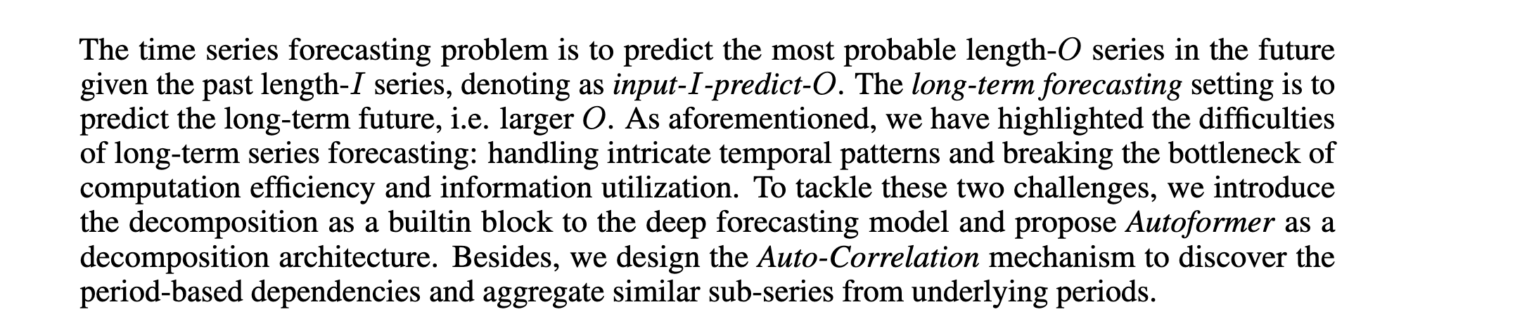
时间序列预测问题是指在给定过去长度为I的时间序列的情况下，预测未来最可能的长度为O的时间序列，记作input-I-predict-O。长期预测设置是指预测长期未来，即O较大。

如前所述，我们已经强调了长期序列预测的难点：处理复杂的时间模式和突破计算效率及信息利用的瓶颈。

为了应对这两个挑战，我们引入分解作为深度预测模型的内置模块，并提出Autoformer作为一种分解架构。

此外，我们设计了自相关机制来发现基于周期的依赖关系，并聚合来自底层周期的相似子序列。

3.1 分解架构

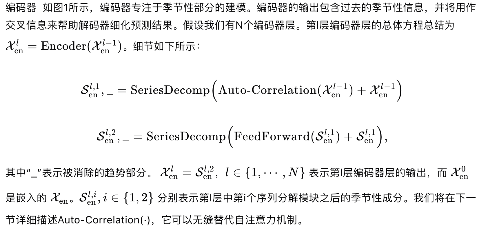
We renovate Transformer [35] to a deep decomposition architecture (Figure 1), including the inner series decomposition block, Auto-Correlation mechanism, and corresponding Encoder and Decoder.

我们对Transformer[35]进行了改造，将其转变为一种深度分解架构（图1），包括内部的序列分解模块、自相关机制以及相应的编码器和解码器。

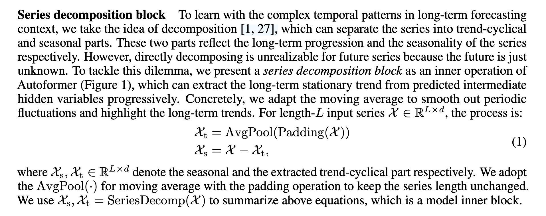
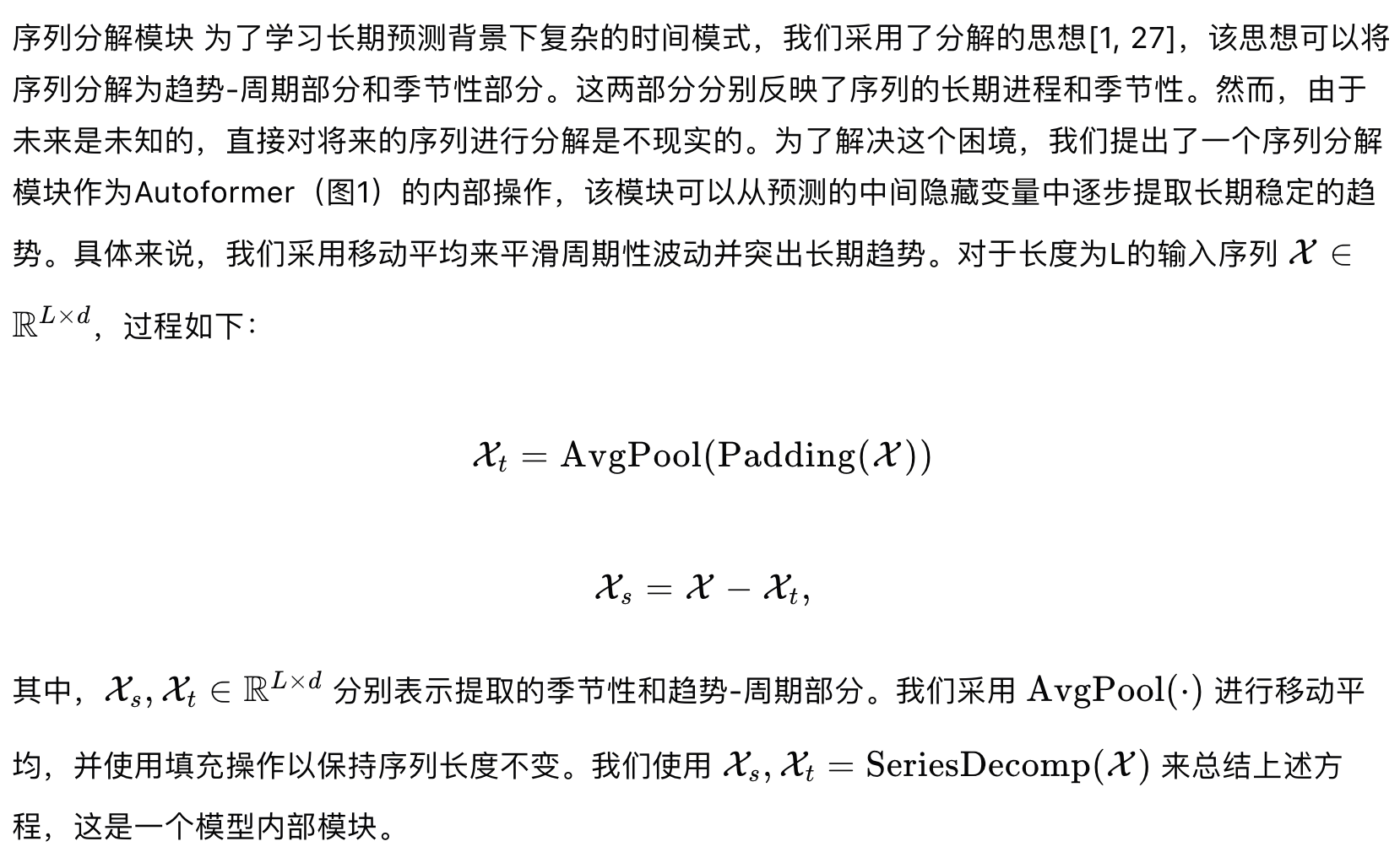
Series decomposition block

代码：

seasonal_init, trend_init = self.decomp(x_enc) # 均为[B, L, D]


self.decomp = series_decomp(kernel_size)

class series_decomp(nn.Module):
    """
    Series decomposition block
    """
    def __init__(self, kernel_size):
        super(series_decomp, self).__init__()
        self.moving_avg = moving_avg(kernel_size, stride=1)

    def forward(self, x):

        # 计算移动平均，提取序列趋势分量
        # x 形状[B, L, D] -> moving_mean形状[B, L, D]
        #  moving_avg内部会进行填充，保证输出形状与输入相同
        moving_mean = self.moving_avg(x)

        # 通过原始序列减去趋势分量，得到残差(季节性分量)，逐元素减法操作
        # x形状[B, L, D] - moving_mean形状[B, L, D] -> res形状[B, L, D]
        res = x - moving_mean

        # 返回季节性分量和趋势分量，均保持原始形状[B, L, D]
        # 第一个返回值res是季节性分量，第二个返回值moving_mean是趋势分量
        return res, moving_mean


class moving_avg(nn.Module):
    """
    Moving average block to highlight the trend of time series
    """
    def __init__(self, kernel_size, stride):
        super(moving_avg, self).__init__()
        self.kernel_size = kernel_size
        self.avg = nn.AvgPool1d(kernel_size=kernel_size, stride=stride, padding=0) # AvgPool1d(kernel_size=(25,), stride=(1,), padding=(0,))

    def forward(self, x):
        # padding on the both ends of time series

        # 提取第一个时间步并重复，用于前端填充 x.shape =  [32, 36, 7]
        #  [B, L, D] -> [B, 1, D] -> [B, (kernel_size-1)//2, D]
        front = x[:, 0:1, :].repeat(1, (self.kernel_size - 1) // 2, 1) 

        # 提取最后一个时间步并重复，用于后端填充
        # [B, L, D] -> [B, 1, D] -> [B, (kernel_size-1)//2, D]
        end = x[:, -1:, :].repeat(1, (self.kernel_size - 1) // 2, 1)

        # 连接填充部分与原序列
        # [B, (k-1)//2, D] + [B, L, D] + [B, (k-1)//2, D] -> [B, L+(k-1), D]
        x = torch.cat([front, x, end], dim=1)

        # 转置并应用一维平均池化
        # [B, L+(k-1), D] -> [B, D, L+(k-1)] -> [B, D, L]
        # 池化窗口大小为kernel_size，步长为1，输出长度为(L+(k-1)-k+1)=L （length + 2P - K + 1）
        x = self.avg(x.permute(0, 2, 1))

        # 转置回原始维度顺序 [B, D, L] -> [B, L, D]
        x = x.permute(0, 2, 1)
        return x

Model inputs

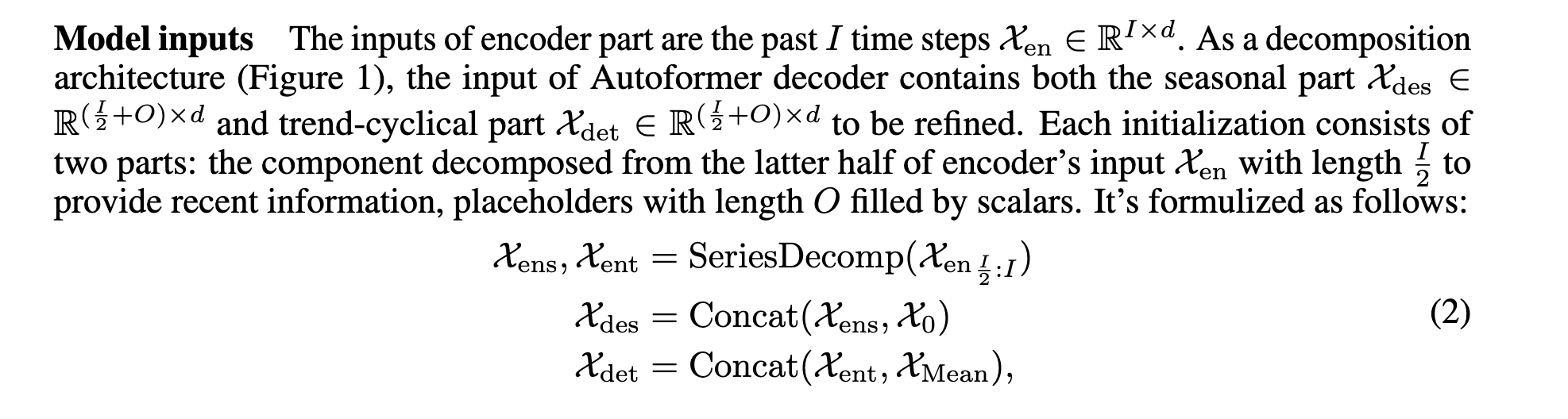
        # decomp init
        # 计算x_enc时间维度平均值，从[B(32), L(36), D(7)]变为[B, 1, D]再扩展为[B, pred_len(24), D]，作为趋势初始值
        mean = torch.mean(x_enc, dim=1).unsqueeze(1).repeat(1, self.pred_len, 1)

        # 创建全零张量 [B, pred_len, D]，用于初始化未来时间步的季节性成分
        zeros = torch.zeros([x_dec.shape[0], self.pred_len, x_dec.shape[2]], device=x_enc.device) 
        # 对输入序列进行时间序列分解，将x_enc[B, L, D]分解为季节性和趋势成分，形状保持不变
        seasonal_init, trend_init = self.decomp(x_enc) # 均为[B, L, D]
     
        # decoder input
        # 解码器趋势输入：连接历史趋势(最后label_len个时间步)和预测趋势初始值
        # 形状变化：[B, label_len, D] + [B, pred_len, D] -> [B, label_len+pred_len, D]
        trend_init = torch.cat([trend_init[:, -self.label_len:, :], mean], dim=1)

        # 解码器季节性输入：连接历史季节性(最后label_len个时间步)和全零预测初始值
        # 形状变化：[B, label_len, D] + [B, pred_len, D] -> [B, label_len+pred_len, D]
        seasonal_init = torch.cat([seasonal_init[:, -self.label_len:, :], zeros], dim=1)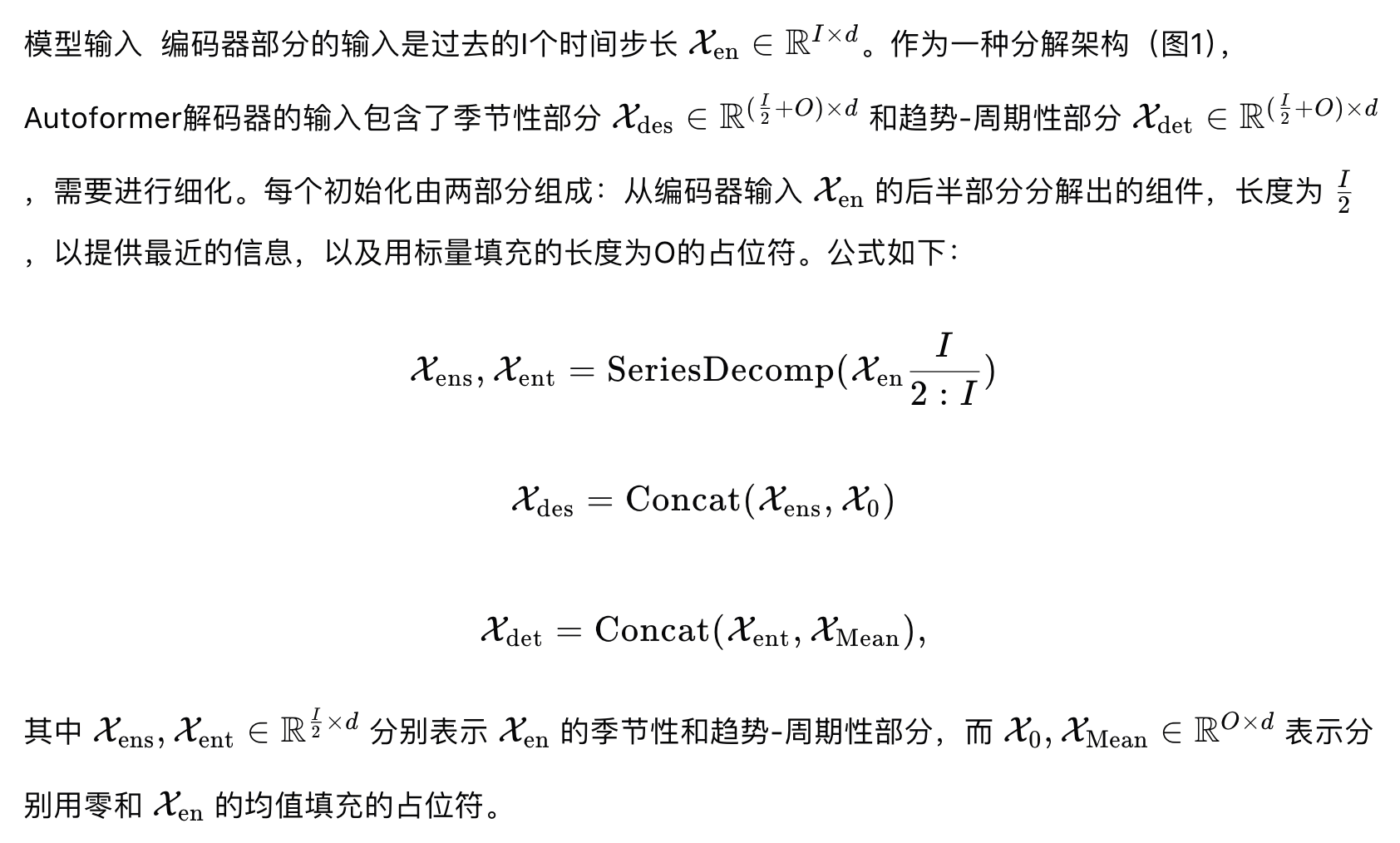

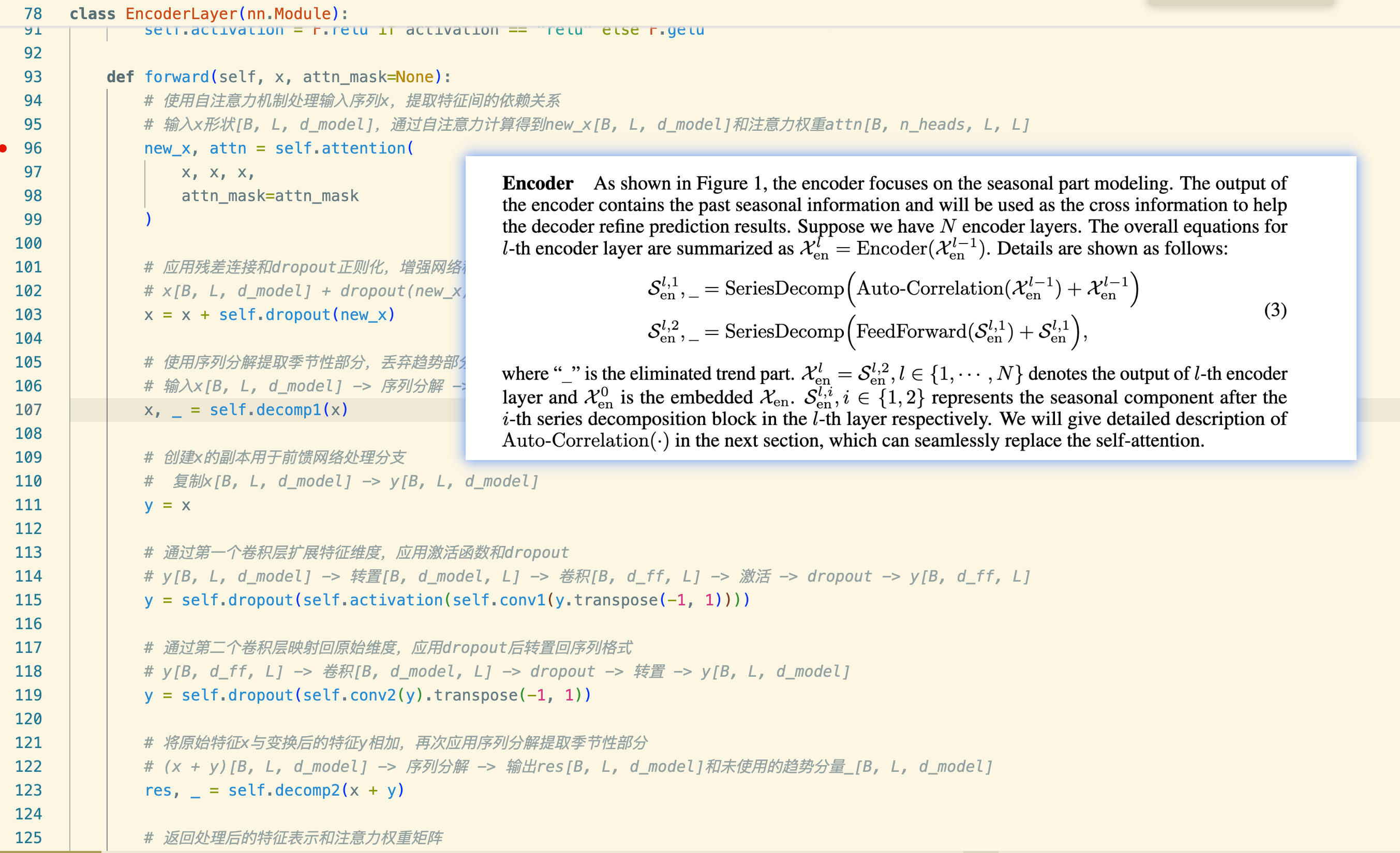
Encoder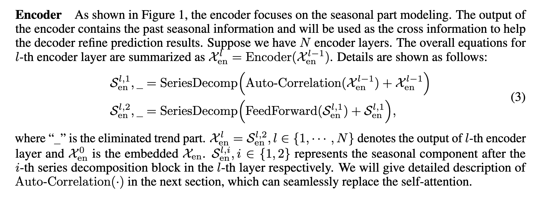

调用关系

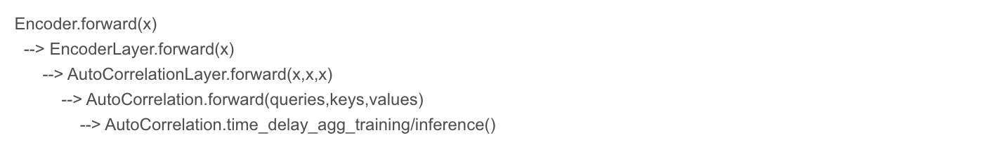
编码器的起点

        # Encoder
        self.encoder = Encoder(
            [
                EncoderLayer(AutoCorrelationLayer(AutoCorrelation(False, configs.factor,attention_dropout=configs.dropout,output_attention=configs.output_attention),configs.d_model, configs.n_heads),
                    configs.d_model,
                    configs.d_ff,
                    moving_avg=configs.moving_avg,
                    dropout=configs.dropout,
                    activation=configs.activation
                ) for l in range(configs.e_layers)
            ],
            norm_layer=my_Layernorm(configs.d_model)
        )

x, _ = self.decomp1(x)

        new_x, attn = self.attention(
            x, x, x,
            attn_mask=attn_mask
        )

        # 应用残差连接和dropout正则化，增强网络稳定性和鲁棒性
        # x[B, L, d_model] + dropout(new_x)[B, L, d_model] -> x[B, L, d_model]        
        x = x + self.dropout(new_x)

res, _ = self.decomp2(x + y)

y 是全连接

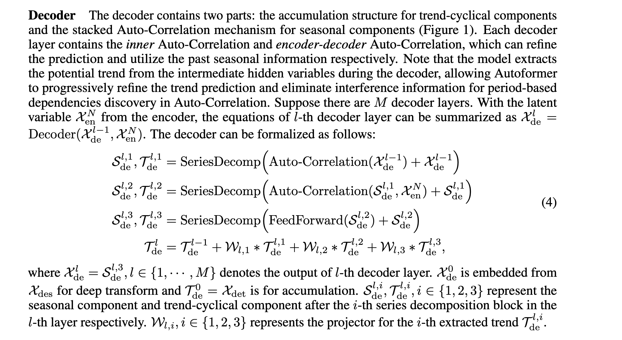
解码器

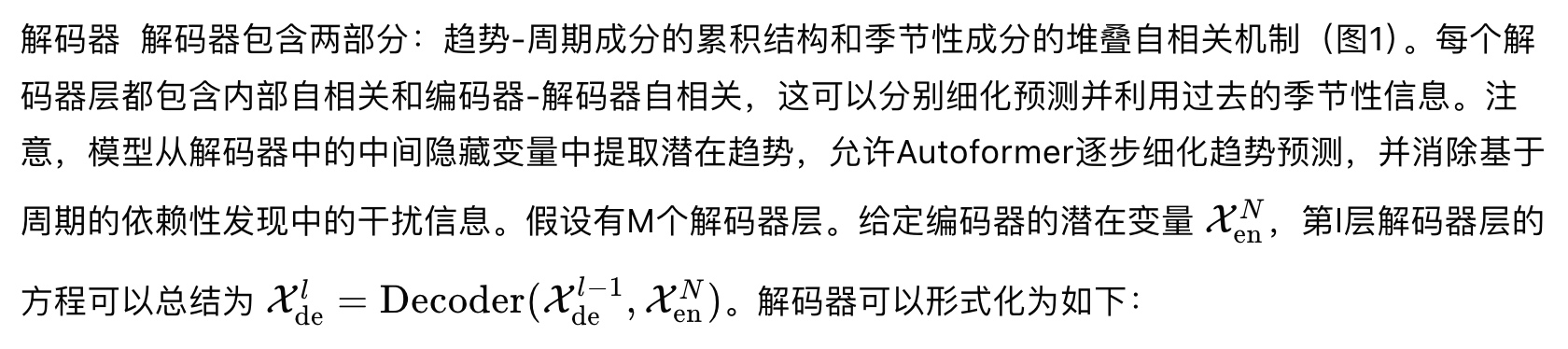
解码器代码

起点

        # Decoder
        self.decoder = Decoder(
            [
                DecoderLayer(
                    AutoCorrelationLayer(
                        AutoCorrelation(True, configs.factor, attention_dropout=configs.dropout,
                                        output_attention=False),
                        configs.d_model, configs.n_heads),
                    AutoCorrelationLayer(
                        AutoCorrelation(False, configs.factor, attention_dropout=configs.dropout,
                                        output_attention=False),
                        configs.d_model, configs.n_heads),
                    configs.d_model,
                    configs.c_out,
                    configs.d_ff,
                    moving_avg=configs.moving_avg,
                    dropout=configs.dropout,
                    activation=configs.activation,
                )
                for l in range(configs.d_layers)
            ],

解码器嵌入以后就调用

      self.dec_embedding = DataEmbedding_wo_pos(configs.dec_in, configs.d_model, configs.embed, configs.freq,
                                                  configs.dropout)  
      dec_out = self.dec_embedding(seasonal_init, x_mark_dec)

        # 通过解码器处理序列，同时利用编码器输出和趋势信息，生成季节性和趋势预测
        # seasonal_part和trend_part均为[B, label_len+pred_len, D]
        seasonal_part, trend_part = self.decoder(dec_out, enc_out, x_mask=dec_self_mask, cross_mask=dec_enc_mask,
                                                 trend=trend_init)

Decoder.forward

class Decoder(nn.Module):
    """
    Autoformer encoder
    """
    def __init__(self, layers, norm_layer=None, projection=None):
        super(Decoder, self).__init__()
        self.layers = nn.ModuleList(layers)
        self.norm = norm_layer
        self.projection = projection

    def forward(self, x, cross, x_mask=None, cross_mask=None, trend=None):
        # 遍历每个解码器层，处理输入序列x和交叉序列cross
        # x[B, L, d_model] -> DecoderLayer.forward -> x[B, L, d_model], residual_trend[B, L, c_out]
        for layer in self.layers:
            # 调用解码器层的前向传播方法，更新x和残差趋势
            # x[B, L, d_model], cross[B, L, d_model] -> DecoderLayer.forward -> x[B, L, d_model], residual_trend[B, L, c_out]
            x, residual_trend = layer(x, cross, x_mask=x_mask, cross_mask=cross_mask)
            # 更新趋势信息，将残差趋势添加到当前趋势
            # trend[B, L, c_out] + residual_trend[B, L, c_out] -> trend[B, L, c_out]
            trend = trend + residual_trend

        # 如果存在归一化层，则对输出进行归一化处理
        # x[B, L, d_model] -> LayerNorm -> x[B, L, d_model]
        if self.norm is not None:
            x = self.norm(x)

        # 如果存在投影层，则对输出进行投影处理
        # x[B, L, d_model] -> Linear -> x[B, L, c_out]
        if self.projection is not None:
            x = self.projection(x)
        # 返回解码器输出和趋势信息
        # 返回值: x[B, L, c_out], trend[B, L, c_out]
        return x, trend

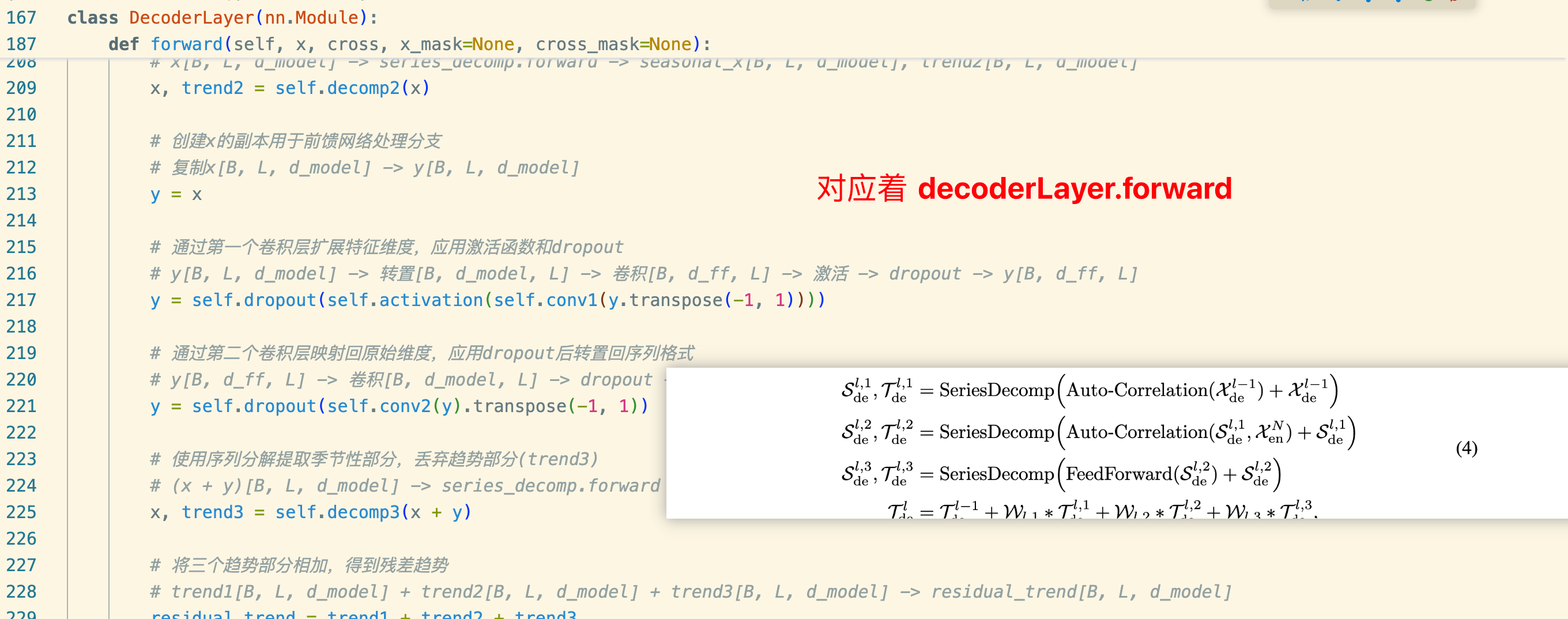
DecoderLayer.forward

class DecoderLayer(nn.Module):
    """
    Autoformer decoder layer with the progressive decomposition architecture
    """
    def __init__(self, self_attention, cross_attention, d_model, c_out, d_ff=None,
                 moving_avg=25, dropout=0.1, activation="relu"):
        super(DecoderLayer, self).__init__()
        d_ff = d_ff or 4 * d_model
        self.self_attention = self_attention
        self.cross_attention = cross_attention
        self.conv1 = nn.Conv1d(in_channels=d_model, out_channels=d_ff, kernel_size=1, bias=False)
        self.conv2 = nn.Conv1d(in_channels=d_ff, out_channels=d_model, kernel_size=1, bias=False)
        self.decomp1 = series_decomp(moving_avg)
        self.decomp2 = series_decomp(moving_avg)
        self.decomp3 = series_decomp(moving_avg)
        self.dropout = nn.Dropout(dropout)
        self.projection = nn.Conv1d(in_channels=d_model, out_channels=c_out, kernel_size=3, stride=1, padding=1,
                                    padding_mode='circular', bias=False)
        self.activation = F.relu if activation == "relu" else F.gelu

    def forward(self, x, cross, x_mask=None, cross_mask=None):

        # 使用自注意力机制处理输入序列x，提取特征间的依赖关系
        # x[B, L, d_model] -> self_attention.forward -> new_x[B, L, d_model]
        x = x + self.dropout(self.self_attention(
            x, x, x,
            attn_mask=x_mask
        )[0])

        # 使用序列分解提取季节性部分，丢弃趋势部分(trend1)
        # x[B, L, d_model] -> series_decomp.forward -> seasonal_x[B, L, d_model], trend1[B, L, d_model]
        x, trend1 = self.decomp1(x)

        # 使用交叉注意力机制处理输入序列x和交叉序列cross，提取特征间的依赖关系
         # x[B, L, d_model], cross[B, L, d_model] -> cross_attention.forward -> new_x[B, L, d_model]
        x = x + self.dropout(self.cross_attention(
            x, cross, cross,
            attn_mask=cross_mask
        )[0])

        # 使用序列分解提取季节性部分，丢弃趋势部分(trend2)
        # x[B, L, d_model] -> series_decomp.forward -> seasonal_x[B, L, d_model], trend2[B, L, d_model]
        x, trend2 = self.decomp2(x)

        # 创建x的副本用于前馈网络处理分支
        # 复制x[B, L, d_model] -> y[B, L, d_model]
        y = x

        # 通过第一个卷积层扩展特征维度，应用激活函数和dropout
        # y[B, L, d_model] -> 转置[B, d_model, L] -> 卷积[B, d_ff, L] -> 激活 -> dropout -> y[B, d_ff, L]
        y = self.dropout(self.activation(self.conv1(y.transpose(-1, 1))))
        
        # 通过第二个卷积层映射回原始维度，应用dropout后转置回序列格式
        # y[B, d_ff, L] -> 卷积[B, d_model, L] -> dropout -> 转置 -> y[B, L, d_model]
        y = self.dropout(self.conv2(y).transpose(-1, 1))

        # 使用序列分解提取季节性部分，丢弃趋势部分(trend3)
        # (x + y)[B, L, d_model] -> series_decomp.forward -> seasonal_x[B, L, d_model], trend3[B, L, d_model]
        x, trend3 = self.decomp3(x + y)

        # 将三个趋势部分相加，得到残差趋势
        # trend1[B, L, d_model] + trend2[B, L, d_model] + trend3[B, L, d_model] -> residual_trend[B, L, d_model]
        residual_trend = trend1 + trend2 + trend3
        
        # 对残差趋势进行投影，调整维度
        # residual_trend[B, L, d_model] -> 转置[B, d_model, L] -> 卷积[B, c_out, L] -> 转置 -> residual_trend[B, L, c_out]
        residual_trend = self.projection(residual_trend.permute(0, 2, 1)).transpose(1, 2)
        
        # 返回处理后的特征表示和残差趋势
        # 返回值: x[B, L, d_model], residual_trend[B, L, c_out]
        return x, residual_trend

AutoCorrelation.forward

AutoCorrelationLayer.forward

图 1

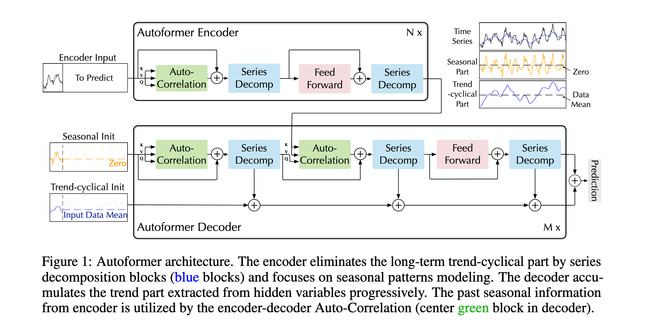
图 1 展示了Autoformer模型的架构，它是一个用于时间序列预测的深度学习模型。该模型由编码器（Encoder）和解码器（Decoder）组成，专门设计来处理长期时间序列预测问题。下面是对图中各部分的详细解释：

编码器部分（Autoformer Encoder）

输入：编码器接收过去I个时间步长的数据作为输入，标记为“Encoder Input”。
自相关机制（Auto-Correlation）：编码器首先通过自相关机制来捕捉时间序列中的周期性依赖。这一步帮助模型理解数据的季节性模式。
序列分解（Series Decomp）：接着，编码器使用序列分解块来分离时间序列的趋势-周期部分和季节性部分。这些分解块以蓝色表示。
前馈网络（Feed Forward）：分解后的数据通过前馈网络进一步处理。
输出：编码器的输出是处理过的季节性信息，这些信息将被用作解码器中的交叉信息，以帮助细化预测结果。

解码器部分（Autoformer Decoder）

初始化：解码器开始时有两个初始化输入，一个是季节性初始化（Seasonal Init），另一个是趋势-周期初始化（Trend-cyclical Init）。这些初始化帮助模型在预测过程中保持时间序列的结构。
自相关机制（Auto-Correlation）：解码器中也包含自相关机制，用于进一步细化预测并利用编码器中提取的季节性信息。
序列分解（Series Decomp）：解码器中的序列分解块用于逐步累积从隐藏变量中提取的趋势部分，并消除周期性依赖的干扰。
前馈网络（Feed Forward）：这些块的输出通过前馈网络进一步处理。
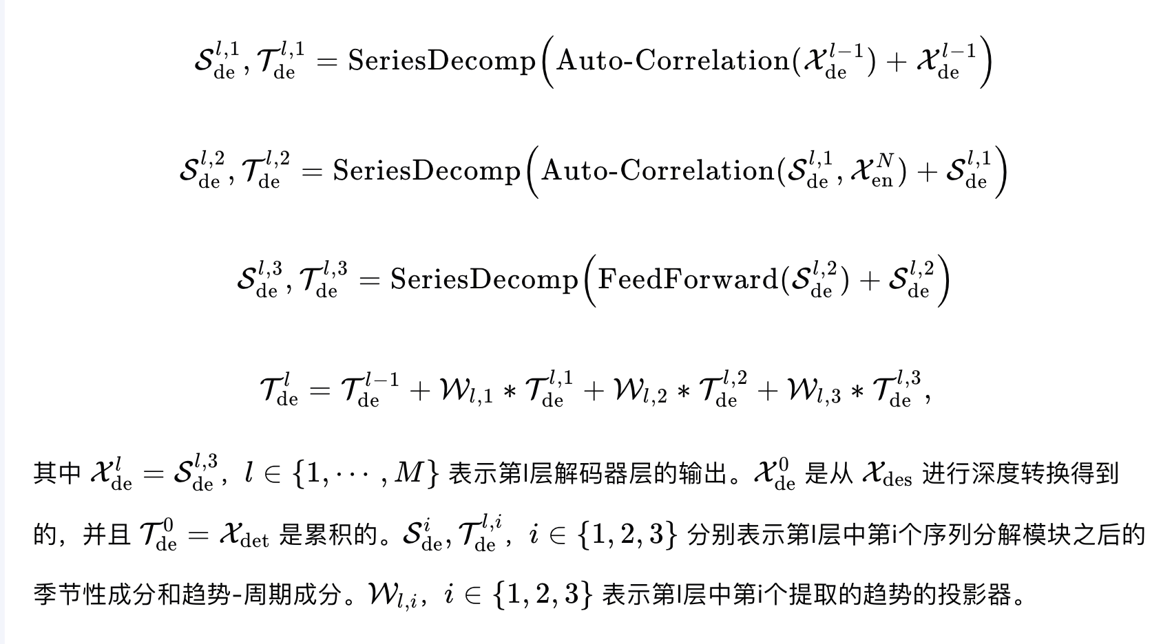
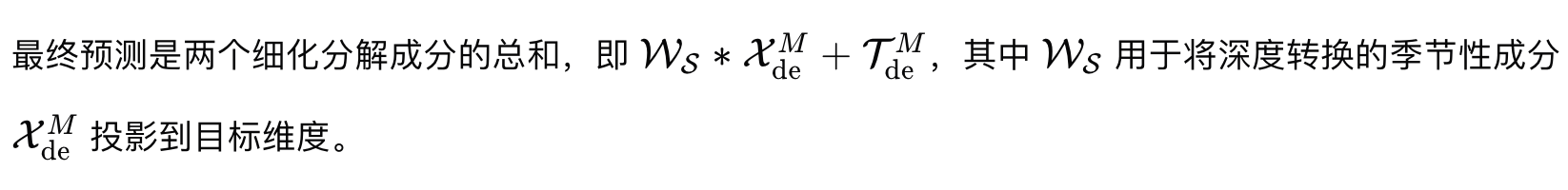
输出：解码器的最终输出是预测的时间序列，它是通过将季节性部分和趋势-周期部分相加得到的。

总结

季节性部分（Seasonal Part）：用黄色表示，代表时间序列中的季节性变化。
趋势-周期部分（Trend-cyclical Part）：用蓝色表示，代表时间序列中的长期趋势和周期性变化。
数据均值（Data Mean）：用灰色表示，是时间序列的平均值，用于初始化和最终预测。

图1展示了Autoformer如何通过编码器-解码器架构和自相关机制来处理和预测时间序列数据，特别是在长期预测设置中。这种设计使得Autoformer能够有效地捕捉时间序列的季节性和趋势性特征，从而提高预测的准确性。

Figure 1: Autoformer architecture. The encoder eliminates the long-term trend-cyclical part by series decomposition blocks (blue blocks) and focuses on seasonal patterns modeling. The decoder accumulates the trend part extracted from hidden variables progressively. The past seasonal information from encoder is utilized by the encoder-decoder Auto-Correlation (center green block in decoder).

图1：Autoformer架构。编码器通过序列分解模块（蓝色模块）消除长期趋势-周期部分，并专注于季节性模式建模。解码器逐步累积从隐藏变量中提取的趋势部分。编码器-解码器自相关机制（解码器中中间的绿色模块）利用了编码器中过去的季节性信息。