


 本文介绍了如何使用Keras库加载预训练的VGG16模型对图像进行分类,包括数据预处理、模型预测以及两种不同模型结构的应用。作者展示了如何使用卷积神经网络进行猫咪、狗狗和熊猫的分类,并展示了模型在不同图片上的识别效果。
from keras.models import load_model
import argparse
import pickle
import cv2
#--image images/dog.jpg --model output/simple\_nn.model --label-bin output/simple\_nn\_lb.pickle --width 32 --height 32 --flatten 1
#--image images/dog.jpg --model output\_cnn/vggnet.model --label-bin output\_cnn/vggnet\_lb.pickle --width 64 --height 64
# 设置输入参数
ap = argparse.ArgumentParser()
ap.add_argument("-i", "--image", required=True,
	help="path to input image we are going to classify")
ap.add_argument("-m", "--model", required=True,
	help="path to trained Keras model")
ap.add_argument("-l", "--label-bin", required=True,
	help="path to label binarizer")
ap.add_argument("-w", "--width", type=int, default=28,
	help="target spatial dimension width")
ap.add_argument("-e", "--height", type=int, default=28,
	help="target spatial dimension height")
ap.add_argument("-f", "--flatten", type=int, default=-1,
	help="whether or not we should flatten the image")
args = vars(ap.parse_args())

# 加载测试数据并进行相同预处理操作
image = cv2.imread(args["image"])
output = image.copy()
image = cv2.resize(image, (args["width"], args["height"]))

# scale the pixel values to [0, 1]
image = image.astype("float") / 255.0
# 是否要对图像就行拉平操作
if args["flatten"] > 0:
	image = image.flatten()
	image = image.reshape((1, image.shape[0]))
# CNN的时候需要原始图像
else:
	image = image.reshape((1, image.shape[0], image.shape[1],
		image.shape[2]))
# 读取模型和标签
print("[INFO] loading network and label binarizer...")
model = load_model(args["model"])
lb = pickle.loads(open(args["label\_bin"], "rb").read())

# 预测
preds = model.predict(image)

i = preds.argmax(axis=1)[0]
label = lb.classes_[i]

text = "{}: {:.2f}%".format(label, preds[0][i] \* 100)
cv2.putText(output, text, (10, 30), cv2.FONT_HERSHEY_SIMPLEX, 0.7,
	(0, 0, 255), 2)

cv2.imshow("Image", output)
cv2.waitKey(0)
这里就是我们预测函数,训练模型我们已经训练好了!然后走一遍前向传播。结果是这样的!

这个分类模型主要用了VGG16,然后我们主要是做猫,狗,熊猫三种分类!

然后我又找了一个猫和老鼠里面的tom猫的照片。然后我们一起来看一下效果!

检测效果非常nice!!!
然后呢我又用了自己女朋友的照片试了一下!

果然!!!果然是这样!!!
训练模块
from sklearn.preprocessing import LabelBinarizer
from sklearn.model_selection import train_test_split
from sklearn.metrics import classification_report#综合结果对比
from keras.models import Sequential
from keras.layers import Dropout
from keras.layers.core import Dense
from keras.optimizers import SGD
from keras import initializers#初始化权重参数
from keras import regularizers#正则化
from my_utils import utils_paths#图像路径的操作
import matplotlib.pyplot as plt
import numpy as np
import argparse
import random
import pickle
import cv2
import os
#--dataset --model --label-bin --plot
# 输入参数
ap = argparse.ArgumentParser()
ap.add_argument("-d", "--dataset", required=True,
	help="path to input dataset of images")
ap.add_argument("-m", "--model", required=True,
	help="path to output trained model")
ap.add_argument("-l", "--label-bin", required=True,
	help="path to output label binarizer")
ap.add_argument("-p", "--plot", required=True,
	help="path to output accuracy/loss plot")
args = vars(ap.parse_args())


print("[INFO] 开始读取数据")
data = []
labels = []

# 拿到图像数据路径,方便后续读取
imagePaths = sorted(list(utils_paths.list_images(args["dataset"])))
random.seed(42)
random.shuffle(imagePaths)

# 遍历读取数据
for imagePath in imagePaths:
	# 读取图像数据,由于使用神经网络,需要给定成一维
	image = cv2.imread(imagePath)
	image = cv2.resize(image, (32, 32)).flatten()
	data.append(image)

	# 读取标签
	label = imagePath.split(os.path.sep)[-2]
	labels.append(label)

# scale图像数据
data = np.array(data, dtype="float") / 255.0
labels = np.array(labels)

# 数据集切分
(trainX, testX, trainY, testY) = train_test_split(data,
	labels, test_size=0.25, random_state=42)

# 转换标签,one-hot格式
lb = LabelBinarizer()
trainY = lb.fit_transform(trainY)
testY = lb.transform(testY)

# 网络模型结构:3072-512-256-3
model = Sequential()
# kernel\_regularizer=regularizers.l2(0.01)
# keras.initializers.TruncatedNormal(mean=0.0, stddev=0.05, seed=None)
# initializers.random\_normal
# #model.add(Dropout(0.8))
model.add(Dense(512, input_shape=(3072,), activation="relu" ,kernel_initializer = initializers.TruncatedNormal(mean=0.0, stddev=0.05, seed=None),kernel_regularizer=regularizers.l2(0.01)))
model.add(Dropout(0.5))
model.add(Dense(256, activation="relu",kernel_initializer = initializers.TruncatedNormal(mean=0.0, stddev=0.05, seed=None),kernel_regularizer=regularizers.l2(0.01)))
model.add(Dropout(0.5))
model.add(Dense(len(lb.classes_), activation="softmax",kernel_initializer = initializers.TruncatedNormal(mean=0.0, stddev=0.05, seed=None),kernel_regularizer=regularizers.l2(0.01)))

# 初始化参数
INIT_LR = 0.001
EPOCHS = 200

# 给定损失函数和评估方法
print("[INFO] 准备训练网络...")
opt = SGD(lr=INIT_LR)
model.compile(loss="categorical\_crossentropy", optimizer=opt,
	metrics=["accuracy"])

# 训练网络模型
H = model.fit(trainX, trainY, validation_data=(testX, testY),
	epochs=EPOCHS, batch_size=32)

# 测试网络模型
print("[INFO] 正在评估模型")
predictions = model.predict(testX, batch_size=32)
print(classification_report(testY.argmax(axis=1),
	predictions.argmax(axis=1), target_names=lb.classes_))

# 当训练完成时,绘制结果曲线
N = np.arange(0, EPOCHS)
plt.style.use("ggplot")
plt.figure()
#plt.plot(N[150:], H.history["loss"][150:], label="train\_loss")
#plt.plot(N[150:], H.history["val\_loss"][150:], label="val\_loss")
plt.plot(N[150:], H.history["accuracy"][150:], label="train\_acc")
plt.plot(N[150:], H.history["val\_accuracy"][150:], label="val\_acc")
plt.title("Training Loss and Accuracy (Simple NN)")
plt.xlabel("Epoch #")
plt.ylabel("Loss/Accuracy")
plt.legend()
plt.savefig(args["plot"])

# 保存模型到本地
print("[INFO] 正在保存模型")
model.save(args["model"])
f = open(args["label\_bin"], "wb")
f.write(pickle.dumps(lb))
f.close()
这里的卷积过程我们直接用vgg16这个来做了。
VGG
from model_name.simple_vggnet import SimpleVGGNet
from sklearn.preprocessing import LabelBinarizer
from sklearn.model_selection import train_test_split
from sklearn.metrics import classification_report
from keras.optimizers import SGD
from keras.preprocessing.image import ImageDataGenerator
from my_utils import utils_paths
import matplotlib.pyplot as plt
import numpy as np
import argparse
import random
import pickle
import cv2
import os
import warnings
warnings.filterwarnings("ignore")

# 设置参数
ap = argparse.ArgumentParser()
ap.add_argument("-d", "--dataset", required=True,
	help="path to input dataset of images")
ap.add_argument("-m", "--model", required=True,
	help="path to output trained model")
ap.add_argument("-l", "--label-bin", required=True,
	help="path to output label binarizer")
ap.add_argument("-p", "--plot", required=True,
	help="path to output accuracy/loss plot")
args = vars(ap.parse_args())

# 读取数据和标签
print("[INFO] loading images...")
data = []
labels = []

# 拿到路径
imagePaths = sorted(list(utils_paths.list_images(args["dataset"])))
random.seed(42)
random.shuffle(imagePaths)

# 读取数据
for imagePath in imagePaths:
	image = cv2.imread(imagePath)
	image = cv2.resize(image, (64, 64))
	data.append(image)
	label = imagePath.split(os.path.sep)[-2]
	labels.append(label)

# 预处理
data = np.array(data, dtype="float") / 255.0
labels = np.array(labels)

# 数据集切分
(trainX, testX, trainY, testY) = train_test_split(data,
	labels, test_size=0.25, random_state=42)

# 标签转换
lb = LabelBinarizer()
trainY = lb.fit_transform(trainY)
testY = lb.transform(testY)

# 数据增强

# aug = ImageDataGenerator(rotation\_range=30, width\_shift\_range=0.1,
# height\_shift\_range=0.1, shear\_range=0.2, zoom\_range=0.2,
# horizontal\_flip=True, fill\_mode="nearest")

# 建立卷积神经网络
model = SimpleVGGNet.build(width=64, height=64, depth=3,
	classes=len(lb.classes_))

# 初始化超参数
INIT_LR = 0.01
EPOCHS = 30
BS = 32

# 损失函数
print("[INFO] 训练网络...")
opt = SGD(lr=INIT_LR, decay=INIT_LR / EPOCHS)
model.compile(loss="categorical\_crossentropy", optimizer=opt,
	metrics=["accuracy"])

# 训练网络

# H = model.fit\_generator(aug.flow(trainX, trainY, batch\_size=BS),
# validation\_data=(testX, testY), steps\_per\_epoch=len(trainX) // BS,
# epochs=EPOCHS)

H = model.fit(trainX, trainY, validation_data=(testX, testY),
	epochs=EPOCHS, batch_size=32)


# 测试
print("[INFO] 测试网络...")
predictions = model.predict(testX, batch_size=32)
print(classification_report(testY.argmax(axis=1),
	predictions.argmax(axis=1), target_names=lb.classes_))

# 展示结果
N = np.arange(0, EPOCHS)
plt.style.use("ggplot")
plt.figure()
plt.plot(N, H.history["loss"], label="train\_loss")
plt.plot(N, H.history["val\_loss"], label="val\_loss")
plt.plot(N, H.history["accuracy"], label="train\_acc")
plt.plot(N, H.history["val\_accuracy"], label="val\_acc")
plt.title("Training Loss and Accuracy (SmallVGGNet)")
plt.xlabel("Epoch #")
plt.ylabel("Loss/Accuracy")
plt.legend()
plt.savefig(args["plot"])

# 保存模型
print("[INFO] 保存模型...")
model.save(args["model"])
f = open(args["label\_bin"], "wb")
f.write(pickle.dumps(lb))
f.close()

网络架构(VGG16神经网络架构)
每一个卷积过程包括了,卷积层然后后面接上relu层,然后归一化操作,还可以进行dropout(七伤拳),就是随机的杀死一些神经元。这样做可以大大的节省计算的时间,成本。后期我们会继续介绍。结果三层卷积过程,然后连接上一层全连接层,最后使用softmax进行分类就完事。
class SimpleVGGNet:
@staticmethod
def build(width, height, depth, classes):
# 不同工具包颜色通道位置可能不一致
model = Sequential()
inputShape = (height, width, depth)
chanDim = -1
if K.image_data_format() == "channels\_first":
inputShape = (depth, height, width)
chanDim = 1
# CONV => RELU => POOL 在特征图上做卷积
model.add(Conv2D(32, (3, 3), padding="same",
input_shape=inputShape))
model.add(Activation("relu"))
model.add(BatchNormalization(axis=chanDim))
model.add(MaxPooling2D(pool_size=(2, 2)))
#model.add(Dropout(0.25))
# (CONV => RELU) \* 2 => POOL
model.add(Conv2D(64, (3, 3), padding="same"))
model.add(Activation("relu"))
model.add(BatchNormalization(axis=chanDim))
model.add(Conv2D(64, (3, 3), padding="same"))
model.add(Activation("relu"))
model.add(BatchNormalization(axis=chanDim))
**既有适合小白学习的零基础资料,也有适合3年以上经验的小伙伴深入学习提升的进阶课程,涵盖了95%以上大数据知识点,真正体系化!**
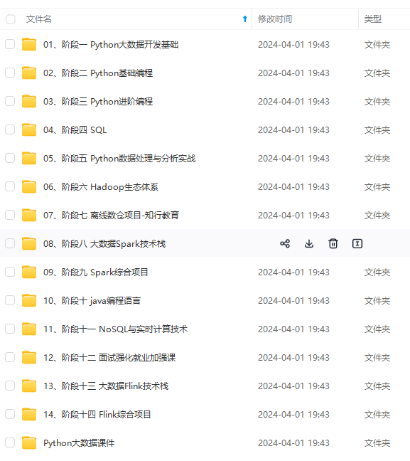
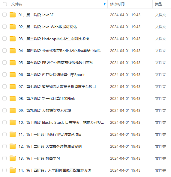
**由于文件比较多,这里只是将部分目录截图出来,全套包含大厂面经、学习笔记、源码讲义、实战项目、大纲路线、讲解视频,并且后续会持续更新**
**[需要这份系统化资料的朋友,可以戳这里获取](https://bbs.csdn.net/topics/618545628)**
atchNormalization(axis=chanDim))
[外链图片转存中...(img-fv1zqqYz-1714738216117)]
[外链图片转存中...(img-4Gh69TiQ-1714738216117)]
[外链图片转存中...(img-sADcAfub-1714738216117)]
**既有适合小白学习的零基础资料,也有适合3年以上经验的小伙伴深入学习提升的进阶课程,涵盖了95%以上大数据知识点,真正体系化!**
**由于文件比较多,这里只是将部分目录截图出来,全套包含大厂面经、学习笔记、源码讲义、实战项目、大纲路线、讲解视频,并且后续会持续更新**
**[需要这份系统化资料的朋友,可以戳这里获取](https://bbs.csdn.net/topics/618545628)**


 533
533

 被折叠的 条评论
为什么被折叠?
被折叠的 条评论
为什么被折叠?
 到【灌水乐园】发言


