基于UNet算法的农业遥感图像语义分割（下）

前言

书接上回，本案例希望建立一个UNET网络模型，来实现对农业遥感图像语义分割的任务。在上篇博文中已经对数据集进行了详细介绍，同时实现了数据筛选、数据集划分等预处理操作，同时对UNET网络模型举了一个详细的例子进行介绍。本篇博客将在处理后的数据集基础上，通过pytorch搭建该网络模型，并实现模型的训练与验证。

1.数据集介绍

为了更好的了解本篇博客，这里对处理后的数据集进行简单的介绍。

1.1文件类型介绍

本篇博客用的数据集在dataset/0.9/目录下，该目录下有两个文件夹和两个文本文档

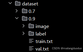
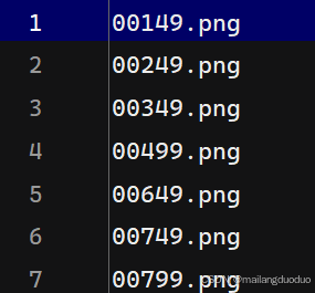
• image:存放原始图像（即模型输入图像）
• label:存放原始图像对应的标签（即语义分割任务的掩码）
• train.txt:每一行代表训练集的图像名称
• val.txt:每一行代表验证集的图像名称
  

注：此处的验证集发挥的功能并不是调整模型超参数的，而是衡量模型的泛化性能，防止过拟合，即测试集的功能。后文所述测试集或者验证集均是代表该文件

1.2数据及标签介绍

数据集（image和label）共计251对原始图像和对应的标签，被划分成训练集（175张）和测试集（76张），即train.txt有175行，val.txt有76行。

• 原始图像：3×512×512，即彩色（三通道）图像
• 标签图像：1×512×512，即单通道灰度图像

每个像素点值表示原始图片中对应位置所属类别，本数据集共计四个类别，分别用像素值0，1，2，3代表。
这里随机选取一对照片进行举例，代码如下：

import matplotlib.pyplot as plt
train=plt.imread('dataset/0.9/image/16213.png')
label=plt.imread('dataset/0.9/label/16213.png')
plt.figure(figsize=(10, 5))
plt.subplot(121)
plt.imshow(train)
plt.axis('off')
plt.subplot(122)
plt.imshow(label)
plt.axis('off')
plt.show()

运行结果：

注：此处使用了matplotlib库中的彩色映射机制进行可视化输出，真实标签值属于集合{0，1，2，3}。

2.UNET网络模型搭建

2.1模型分析

因为原始图像和标签的尺寸大小均为512×512，所以并不能直接使用上篇博客介绍的网络模型。因为该网络结构输入图像尺寸为1×572×572的单通道图像，经过网络模型处理，得到的输出为2×388×388的双通道图像，属于二分类的语义分割模型，和本案例有一定差距。

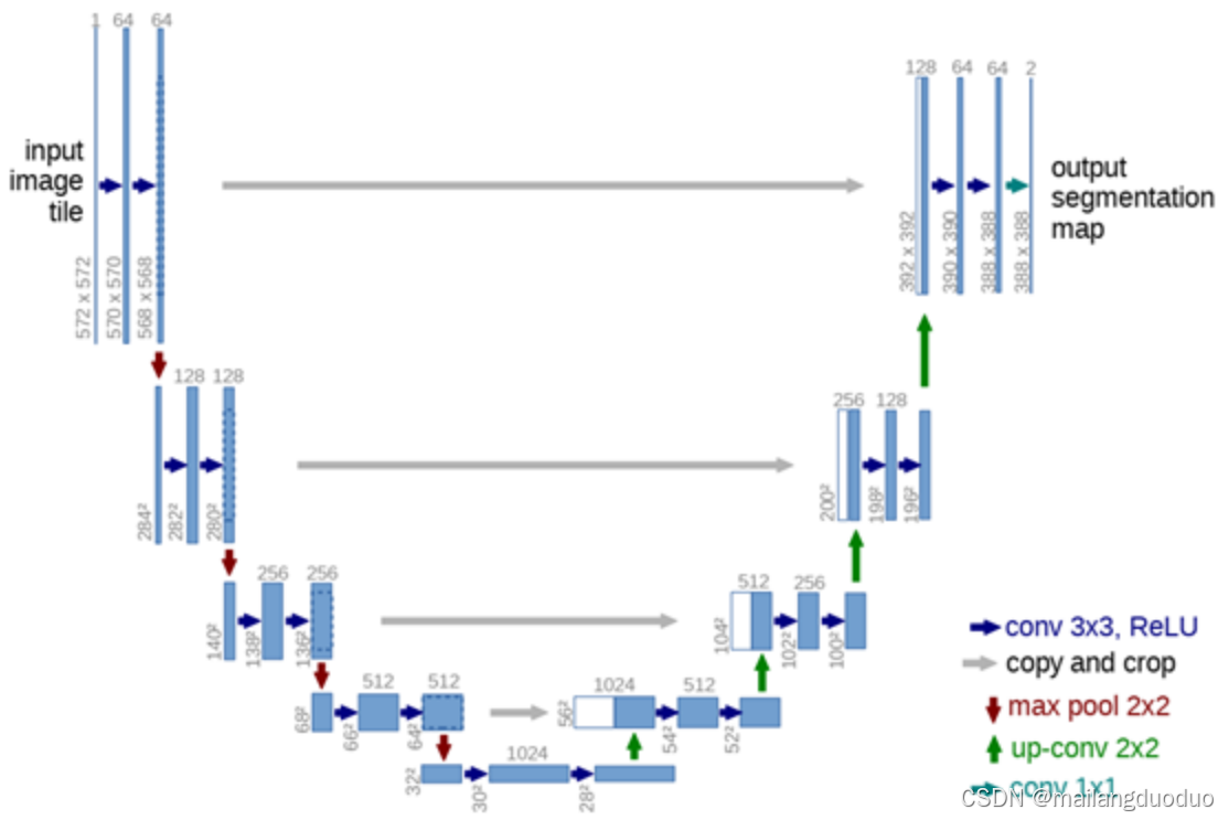
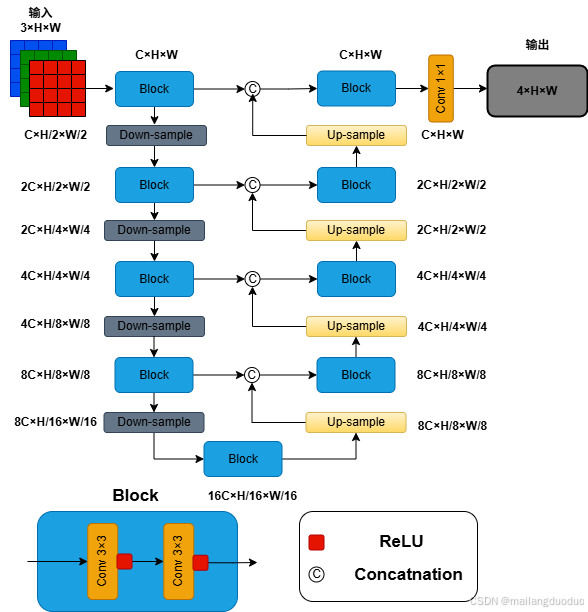
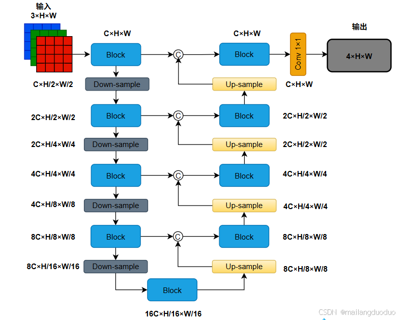
所以，需要对网络模型的输入和输出进行调整。这里为了模块化描述，将上图中的连续两次卷积激活操作封装成了一个Block，同时考虑到标签的尺寸和模型的输入尺寸相同，所以在实际操作中需要padding操作保持图像尺寸大小不变。本案例所使用的网络结构图如下所示：

这里对该结构图做以下补充描述：

• 这里并未减少UNET整体结构，即仍采用四级编码器-解码器架构。为了使模型更好的描述其他尺寸图像作为输入，这里使用了C、H、W分别代表图片的通道数、高度、宽度信息。
• 为了方便理解，图中也对每个输出后的图像尺寸大小进行了标注，此案例中的C在实际模型中数值为32,H、W均为512。
• 为了更好的描述编码器和解码器架构，图示并未标明该架构中下采样和上采样操作采用的具体措施。此案例实际模型中下采样采用最大池化方式，上采样采用转置卷积（反卷积）方式。

2.2模型搭建

2.2.1前提介绍

本案例使用pytorch框架进行模型搭建，在定义网络结构时，一般采用定义类直接继承torch.nn.Module，该类中包含两个方法体：

• __init__方法：用于初始化对象属性，属于面向对象编程范畴。

• forward方法：定义了神经网络模块的前向传播过程，是网络结构中不可或缺的部分。
  注：如果未接触过面向对象编程，建议还是了解一下面向对象的三大特性，可以阅读我早期文章——理解Java中的面向对象，可能表述的并不是太好，因为当时也刚接触。

因此网络模型结构一般如下：

class Block(nn.Module):
    def __init__(self):
        super(Block, self).__init__()
		# 构造方法
    def forward(self, x):
		# 前向传播
        return x

2.2.2Bolck

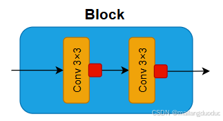
对于该模块，包含两个卷积层和两个 ReLU 激活函数。网络结构可定义如下两种形式：

1. 方式一

class Block(nn.Module):
    def __init__(self, in_channels, out_channels):
        super(Block, self).__init__()
        self.in_channels = in_channels
        self.out_channels = out_channels
    def forward(self, x):
        for i in range(2):
            x = nn.Conv2d(self.in_channels, self.out_channels, kernel_size=3, padding=1)(x)
            x = nn.ReLU(inplace=False)(x)
            self.in_channels = self.out_channels
        return x

2. 方式二

class Block(nn.Module):
    def __init__(self, in_channels, out_channels):
        super(Block, self).__init__()
        self.relu = nn.ReLU(inplace=False)
        self.conv1 = nn.Conv2d(in_channels, out_channels, kernel_size=3, padding=1)
        self.conv2 = nn.Conv2d(out_channels, out_channels, kernel_size=3, padding=1)
    def forward(self, x):
        x=self.conv1(x)
        x=self.relu(x)
        x=self.conv2(x)
        x=self.relu(x)
        return x

上述两种方式等价，后续采用方式二，将卷积、激活等函数声明为一个新的属性。因为采用的是3×3卷积，所以为了保持图像尺寸不发生变化，采用padding=1进行填充。

2.2.3Net模块

Net模块是建立在Block模块基础上进行搭建的，也是整个UNET网络结构的核心。结构示意图如下：

代码实现：

class Net(nn.Module):
    def __init__(self, ):
        super(Net, self).__init__()
        self.relu = nn.ReLU(inplace=False)
        self.pool = nn.MaxPool2d(kernel_size=2, stride=2)
        self.conv1 = Block(3, 32)
        self.conv2 = Block(32, 64)
        self.conv3 = Block(64, 128)
        self.conv4 = Block(128, 256)
        self.conv5 = Block(256, 512)
        self.up6 = nn.ConvTranspose2d(512, 256, kernel_size=2, stride=2)
        self.conv6 = Block(512, 256)
        self.up7 = nn.ConvTranspose2d(256, 128, kernel_size=2, stride=2)
        self.conv7 = Block(256, 128)
        self.up8 = nn.ConvTranspose2d(128, 64, kernel_size=2, stride=2)
        self.conv8 = Block(128, 64)
        self.up9 = nn.ConvTranspose2d(64, 32, kernel_size=2, stride=2)
        self.conv9 = Block(64, 32)
        self.conv10 = nn.Conv2d(32, 4, kernel_size=1)

    def forward(self, x):
        conv1=self.conv1(x) # 32, 512, 512
        # print(conv1.shape)
        pool1=self.pool(conv1)  # 32, 256, 256
        # print(pool1.shape)
        conv2=self.conv2(pool1) # 64, 256, 256
        # print(conv2.shape)
        pool2=self.pool(conv2)  # 64, 128, 128
        # print(pool2.shape)
        conv3=self.conv3(pool2) # 128, 128, 128
        # print(conv3.shape)
        pool3=self.pool(conv3)  # 128, 64, 64
        # print(pool3.shape)
        conv4=self.conv4(pool3) # 256, 64, 64
        # print(conv4.shape)
        pool4=self.pool(conv4)  # 256, 32, 32
        # print(pool4.shape)
        conv5=self.conv5(pool4) # 512, 32, 32
        # print(conv5.shape)
        up6=self.up6(conv5) # 256, 64, 64
        # print(up6.shape)
        conv6=torch.cat([up6,conv4],dim=1)  # 512, 64, 64
        # print(conv6.shape)
        conv6=self.conv6(conv6) # 256, 64, 64
        # print(conv6.shape)
        up7=self.up7(conv6) # 128, 128, 128
        # print(up7.shape)
        conv7=torch.cat([up7,conv3],dim=1)  # 256, 128, 128
        # print(conv7.shape)
        conv7=self.conv7(conv7) # 128, 128, 128
        # print(conv7.shape)
        up8=self.up8(conv7) # 64, 256, 256
        # print(up8.shape)
        conv8=torch.cat([up8,conv2],dim=1)  # 128, 256, 256
        # print(conv8.shape)
        conv8=self.conv8(conv8) # 64, 256, 256
        # print(conv8.shape)
        up9=self.up9(conv8) # 32, 512, 512
        # print(up9.shape)
        conv9=torch.cat([up9,conv1],dim=1)  # 64, 512, 512
        # print(conv9.shape)
        conv9=self.conv9(conv9) # 32, 512, 512
        # print(conv9.shape)
        conv10=self.conv10(conv9)   # 4, 512, 512
        # print(conv10.shape)
        return conv10

在进行编写前向传播forward的时候，可以加一些print()函数来查看形状，没必要像代码所示如此频繁，也可以设置断点进行查看，同时对当前网络前向传播过程中的图片形状做了标注，便于理解。

2.3模型信息查看

这里介绍两种方式：

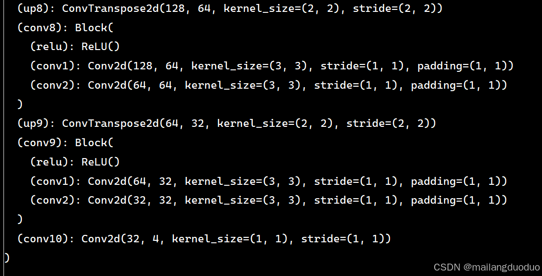
1. 创建实例对象，直接输出即可

if __name__ == "__main__":
    model = Net()
    print(model)

结果如下：

2. 使用get_model_complexity_info函数

if __name__ == "__main__":
    model = Net()
    ops, params = get_model_complexity_info(model, (3,512,512), as_strings=True, print_per_layer_stat=True, verbose=True)
    print(ops, params)
    print('\nTrainable parameters : {}\n'.format(sum(p.numel() for p in model.parameters() if p.requires_grad)))
    print('\nTotal parameters : {}\n'.format(sum(p.numel() for p in model.parameters())))

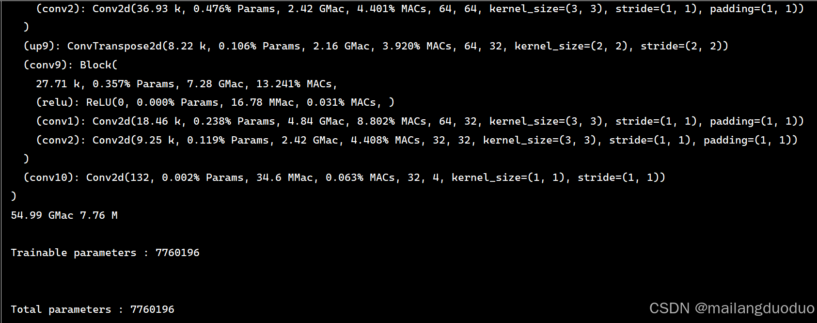
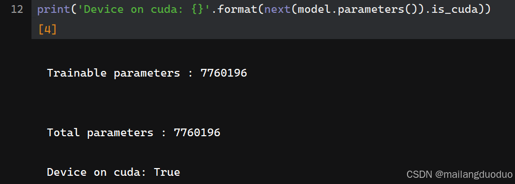
通过结果可以看出，该模型参数量还是相当大的，参数量为7.76M,即776万参数量。

3.模型训练

3.1数据集类的定义

在使用外部的数据集进行模型训练时，一般会定义一个数据集类（ 此处指mydataset），该类继承自 torch.utils.data.Dataset,代码如下：

import numpy as np
from torch.utils.data import Dataset, DataLoader
import cv2
import tqdm
import os
def image_read(train_lines):
    img_list = []
    label_list = []
    for i in tqdm.tqdm(range(len(train_lines))):
        img=cv2.imread(os.path.join('./dataset/0.9/image',train_lines[i][:-1]))
        label=cv2.imread(os.path.join('./dataset/0.9/label',train_lines[i][:-1]))
        label = cv2.cvtColor(label, cv2.COLOR_BGR2GRAY)
        img=np.transpose(img, (2, 0, 1))

        img_list.append(img)
        label_list.append(label)
    return img_list,label_list

class mydataset(Dataset):
    def __init__(self, lines,training=True):
        if training:
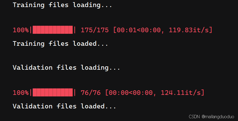
            print('Training files loading...\n')
            self.img_list,self.label_list= image_read(lines)
            print('Training files loaded...\n')
        else:
            print('Validation files loading...\n')
            self.img_list,self.label_list= image_read(lines)
            print('Validation files loaded...\n')
    def __len__(self):
        return len(self.img_list)
    def __getitem__(self, idx):
        img = self.img_list[idx]
        label = self.label_list[idx]
        # 归一化
        img = img / 255.0
        # label = label / 255.0
        return img, label

这里对代码部分做以下说明：

• image_read()函数:将路径中的图片和标签全部加载进来，并以列表的形式返回。这里读取方式使用的是cv2.imread()，该函数返回的图像数组形状是 (H, W, C)，所以使用了np.transpose()函数进行调序；之所以在读取的时候使用train_lines[i][:-1]，是因为每一行读取的时候，最后一个是换行符；因为标签对应的是灰度图，所以读取过后需进行灰度转换。

对于mydataset类

• __init__():用于初始化对象，training=True用于区别数据集和验证集
• __len__():用于返回数据集大小
• __getitem__():用于返回指定下标图片数据，在这里使用了简单粗暴的归一化手段，因为个人觉得label数据本身就很小了，就没有进行归一化处理，当然也可以选择除3（因为标签最大值是3）进行归一化。如果觉得数据集太小，也可以在此处编写数据增强技术（随即裁剪，翻转等）

3.2数据集加载

完成数据集类的定义后，可以使用DataLoader完成数据集的加载。代码如下：

with open('./dataset/0.9/train.txt', 'r') as f:
    train_lines = f.readlines()
with open('./dataset/0.9/val.txt', 'r') as f:
    val_lines = f.readlines()
dataloader_train = DataLoader(mydataset(train_lines,training=True),batch_size=8,shuffle=True)
dataloader_val = DataLoader(mydataset(val_lines,training=False),batch_size=8,shuffle=False)

这里批量大小选择的是8，出于一下考虑：

• 批量大小越小，模型训练阶段的损失越容易波动
• 批量大小越大，完成一次参数更新的时间越长，增加训练时间
• 个人设备显存有限，如果使用cpu训练，那不需要考虑该问题，因为内存会使用页面置换算法将无法容纳的部分置换到硬盘（外存设备）中

另外训练集需要打乱顺序，避免模型学习到顺序相关信息，导致模型泛化性能较差，而测试集无影响，打乱与不打乱均可。
运行结果如下：

接着查看一下，是否加载符合需求，代码如下：

for i, (img, label) in enumerate(dataloader_train):
    print(img.shape)
    print(label.shape)
    break

运行结果：

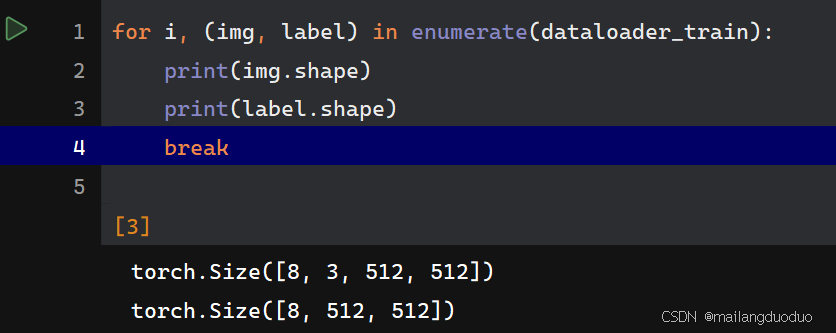
通过结果看出，符合要求。因为批量大小为8，同时输入图片大小3×512×512，输出标签大小512×512。

3.3训练设备选择

在模型训练前，需要选择训练设备是GPU还是CPU，GPU会大大加快速度，可以通过如下指令查看是否成功安装GPU版本的pytorch

import torch
if torch.cuda.is_available():
    print('GPU is available')
else:
    print('GPU is not available')

接着将模型迁移至对应设备，代码如下：

import torch
from Net import Net
if torch.cuda.is_available():
    device = torch.device("cuda")
else:
    device = torch.device("cpu")
model = Net()
model=model.double()
print('\nTrainable parameters : {}\n'.format(sum(p.numel() for p in model.parameters() if p.requires_grad)))
print('\nTotal parameters : {}\n'.format(sum(p.numel() for p in model.parameters())))
model = model.to(device)
print('Device on cuda: {}'.format(next(model.parameters()).is_cuda))

运行结果如下：

3.4模型训练

本案例损失选择交叉熵损失函数，优化器选择Adam，初始学习率为0.0001，并使用tensorboard对训练结果进行可视化输出。代码如下：

import torch
import numpy as np
from tqdm import tqdm
from torch.utils.tensorboard import SummaryWriter

iter_num = 0
getLoss = torch.nn.CrossEntropyLoss()
optimizer = torch.optim.Adam(model.parameters(), lr=0.0001)
optimizer.zero_grad()

# 创建一个 SummaryWriter 对象，用于将数据写入 TensorBoard
writer = SummaryWriter("logs")
epoch=0
while iter_num < 1000:
    epoch+=1
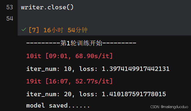
    print("---------第{}轮训练开始---------".format(epoch))
    for i, (img, label) in tqdm(enumerate(dataloader_train)):
        img = img.to(device)
        label = label.long().to(device)
        model.train()
        output = model(img)
        iter_num += 1
        loss = getLoss(output, label)
        loss.backward()
        optimizer.step()
        optimizer.zero_grad()
        if iter_num % 10 == 0:
            print('iter_num: {}, loss: {}'.format(iter_num, loss.item()))
            # 记录训练损失到 TensorBoard
            writer.add_scalar('Training Loss', loss.item(), iter_num)

        if iter_num % 20 == 0:
            torch.save({'model': model.state_dict()},  './models/weights_{}.pth'.format(iter_num))
            print('model saved......')
            with torch.no_grad():
                model.eval()
                losses = []
                for _, (img, label) in tqdm(enumerate(dataloader_val)):
                    img = img.to(device)
                    label = label.long().to(device)
                    output = model(img)
                    loss = getLoss(output, label)
                    losses.append(loss.item())
                val_loss = np.mean(losses)
                print('iter_num: {}, val_loss: {}'.format(iter_num, val_loss))
                # 记录验证损失到 TensorBoard
                writer.add_scalar('Validation Loss', val_loss, iter_num)

writer.close()

这里模型参数信息每更新10次，记录一次损失函数，每更新20次在测试集进行验证统计损失，并保存模型参数。这里测试集验证过于频繁，可以适当调高，加快模型训练。这里由于个人显卡属于低配版-RTX 3050，所以训练时间很长。

训练完成后，对一张图片进行验证模型的分割效果，代码如下

I=cv2.imread('dataset/test.png')
I=np.transpose(I, (2, 0, 1))
I=I/255.0
I=I.reshape(1,3,512,512)
I=torch.tensor(I).to(device)
output=model(I)
output.shape

在输入模型前，需要对图片做出同样的预处理操作，因为模型输入的图片是带有批量大小的，所以使用了reshape()函数。接着将结果进行可视化输出，代码如下：

import matplotlib.pyplot as plt
output=model(I)
predicted_classes = torch.argmax(output, dim=1).squeeze(0).cpu().numpy()

# 创建彩色映射
color_map = {
    0: [0, 0, 0],  # 黑色
    1: [255, 0, 0],  # 红色
    2: [0, 255, 0],  # 绿色
    3: [0, 0, 255]  # 蓝色
}

# 根据预测类别填充颜色
height, width = predicted_classes.shape
colored_image = np.zeros((height, width, 3), dtype=np.uint8)
for i in range(height):
    for j in range(width):
        class_id = predicted_classes[i, j]
        colored_image[i, j] = color_map[class_id]

plt.imshow(colored_image)
plt.axis('off')
plt.show()

运行结果：

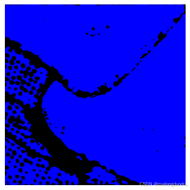
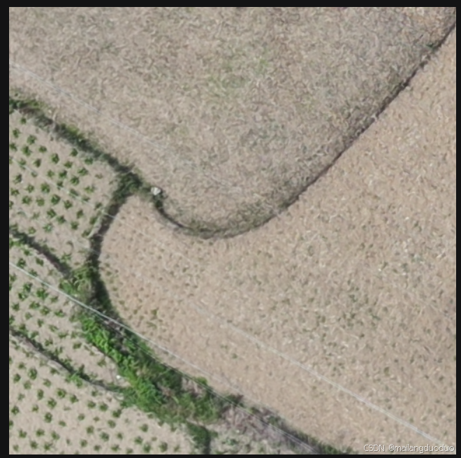
模型输入的图像为：

通过结果可以看出，该分类模型貌似只实现了二分类的语义分割，同时对其他图片也进行了验证，输出图像只有黑色和蓝色，目前个人尚不知道什么原因，求助中…
同时，个人也尝试增加了训练轮数，在上述模型的基础上，增加了400次参数更新，代码如下：

import torch
import numpy as np
from tqdm import tqdm
from torch.utils.tensorboard import SummaryWriter

# 假设 model、dataloader_train、dataloader_val 和 device 已经定义
iter_num = 1000
getLoss = torch.nn.CrossEntropyLoss()
optimizer = torch.optim.Adam(model.parameters(), lr=0.0001)
optimizer.zero_grad()

# 创建一个 SummaryWriter 对象，用于将数据写入 TensorBoard
writer = SummaryWriter("logs")
while iter_num < 1400:
    epoch+=1
    print("---------第{}轮训练开始---------".format(epoch))
    for i, (img, label) in tqdm(enumerate(dataloader_train)):
        img = img.to(device)
        label = label.long().to(device)
        model.train()
        output = model(img)
        iter_num += 1
        loss = getLoss(output, label)
        loss.backward()
        optimizer.step()
        optimizer.zero_grad()
        if iter_num % 10 == 0:
            print('iter_num: {}, loss: {}'.format(iter_num, loss.item()))
            # 记录训练损失到 TensorBoard
            writer.add_scalar('Training Loss', loss.item(), iter_num)

        if iter_num % 40 == 0:
            torch.save({'model': model.state_dict()},  './models/weights_{}.pth'.format(iter_num))
            print('model saved......')
            with torch.no_grad():
                model.eval()
                losses = []
                for _, (img, label) in tqdm(enumerate(dataloader_val)):
                    img = img.to(device)
                    label = label.long().to(device)
                    output = model(img)
                    loss = getLoss(output, label)
                    losses.append(loss.item())
                val_loss = np.mean(losses)
                print('iter_num: {}, val_loss: {}'.format(iter_num, val_loss))
                # 记录验证损失到 TensorBoard
                writer.add_scalar('Validation Loss', val_loss, iter_num)

# 关闭 SummaryWriter
writer.close()

此时模型对该图片的预测效果为：

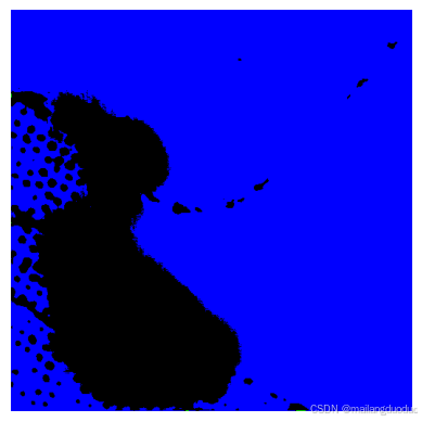
貌似结果好像更差了些，同时对其他图片也进行了验证，输出图像只有黑色和蓝色，仍然属于二分类的语义分割。
在训练过程中的损失曲线如下图所示，个人也不知道什么原因导致如此波动。

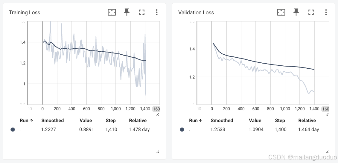
真实训练效果为灰色曲线，黑色曲线平滑和的效果。

4.小结

至此基于UNet算法的农业遥感图像语义分割案例完成，由于个人能力原因，并未接触过实际的项目开发训练过程，所以对于超参数的选择只是基于课本上所学知识，仅供参考。
针对在本案例中出现的两个问题：

1. 为什么模型预测结果属于二分类语义分割的效果，更换其他的图片，同样只有黑色和蓝色？
2. 训练过程中的损失为什么波动这么剧烈？

个人并不知道原因，如有知道什么原因，希望您能告知与我，万分感谢！！！