


一、前言
这一篇续接前一篇《yolo v2之车牌检测后续识别字符(一)》,主要是生成模型文件、配置文件以及训练、测试模型。
二、python接口生成配置文件、模型文件
车牌图片端到端识别的模型文件参考自这里,模型图如下所示:
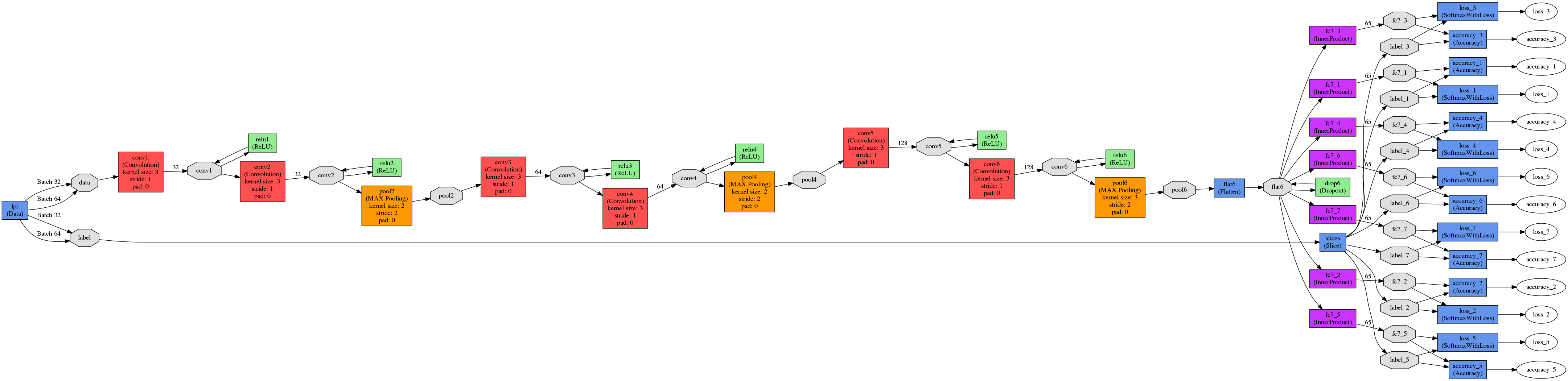
本来想使用caffe的python接口生成prototxt,结果发现很麻烦,容易出错,直接在可视化工具netscope上对已有prototxt做修改更方便,写模型文件时,注意输入的图片、卷积核大小、pad大小、stride大小、输出图片大小的关系,无论卷积层还是池化层,都有
输入:n, c_i, h_i, w_i
输出:n, c_o, h_o, w_o
满足: h_o = ( h_i + 2*pad_h - kernel_h) / stride_h +1
w_o = ( w_i + 2*pad_w - kernel_w ) / stride_w +1
#lpr_train_val.prototxt
name: "Lpr"
layer {
  name: "lpr"
  type: "Data"
  top: "data"
  top: "label"
  include {
    phase: TRAIN
  }
  transform_param {
    scale: 0.00390625
    mean_file: "/home/jyang/caffe/LPR/Mean/mean.binaryproto"
  }
  data_param {
    source: "/home/jyang/caffe/LPR/Build_lmdb/train_lmdb"
    batch_size: 32
    backend: LMDB
  }
}
layer {
  name: "lpr"
  type: "Data"
  top: "data"
  top: "label"
  include {
    phase: TEST
  }
  transform_param {
    scale: 0.00390625
    mean_file: "/home/jyang/caffe/LPR/Mean/mean.binaryproto"
  }
  data_param {
    source: "/home/jyang/caffe/LPR/Build_lmdb/val_lmdb"
    batch_size: 32
    backend: LMDB
  }
}
layer {
  name: "slices"
  type: "Slice"
  bottom: "label"
  top: "label_1"
  top: "label_2"
  top: "label_3"
  top: "label_4"
  top: "label_5"
  top: "label_6"
  top: "label_7"
  slice_param {
    axis: 1
    slice_point: 1
    slice_point: 2
    slice_point: 3
    slice_point: 4
    slice_point: 5
    slice_point: 6
  }
}
layer {
  name: "conv1"
  type: "Convolution"
  bottom: "data"
  top: "conv1"
  param {
    lr_mult: 1
    decay_mult: 1
  }
  param {
    lr_mult: 2
    decay_mult: 0
  }
  convolution_param {
    num_output: 32
    kernel_size: 3
    stride: 1
    weight_filler {
      type: "xavier"
    }
    bias_filler {
      type: "constant"
    }
  }
}
layer {
  name: "relu1"
  type: "ReLU"
  bottom: "conv1"
  top: "conv1"
}
layer {
  name: "conv2"
  type: "Convolution"
  bottom: "conv1"
  top: "conv2"
  param {
    lr_mult: 1
    decay_mult: 1
  }
  param {
    lr_mult: 2
    decay_mult: 0
  }
  convolution_param {
    num_output: 32
    kernel_size: 3
    stride: 1
    weight_filler {
      type: "xavier"
    }
    bias_filler {
      type: "constant"
    }
  }
}
layer {
  name: "relu2"
  type: "ReLU"
  bottom: "conv2"
  top: "conv2"
}
layer {
  name: "pool2"
  type: "Pooling"
  bottom: "conv2"
  top: "pool2"
  pooling_param {
    pool: MAX
    kernel_size: 2
    stride: 2
  }
}
layer {
  name: "conv3"
  type: "Convolution"
  bottom: "pool2"
  top: "conv3"
  param {
    lr_mult: 1
    decay_mult: 0
  }
  param {
    lr_mult: 2
    decay_mult: 0
  }
  convolution_param {
    num_output: 64
    kernel_size: 3
    stride: 1
    weight_filler {
      type: "xavier"
    }
    bias_filler {
      type: "constant"
    }
  }
}
layer {
  name: "relu3"
  type: "ReLU"
  bottom: "conv3"
  top: "conv3"
}
layer {
  name: "conv4"
  type: "Convolution"
  bottom: "conv3"
  top: "conv4"
  param {
    lr_mult: 1
    decay_mult: 0
  }
  param {
    lr_mult: 2
    decay_mult: 0
  }
  convolution_param {
    num_output: 64
    kernel_size: 3
    stride: 1
    weight_filler {
      type: "xavier"
    }
    bias_filler {
      type: "constant"
    }
  }
}
layer {
  name: "relu4"
  type: "ReLU"
  bottom: "conv4"
  top: "conv4"
}
layer {
  name: "pool4"
  type: "Pooling"
  bottom: "conv4"
  top: "pool4"
  pooling_param {
    pool: MAX
    kernel_size: 2
    stride: 2
  }
}
layer {
  name: "conv5"
  type: "Convolution"
  bottom: "pool4"
  top: "conv5"
  param {
    lr_mult: 1
    decay_mult: 0
  }
  param {
    lr_mult: 2
    decay_mult: 0
  }
  convolution_param {
    num_output: 128
    kernel_size: 3
    stride: 1
    weight_filler {
      type: "xavier"
    }
    bias_filler {
      type: "constant"
    }
  }
}
layer {
  name: "relu5"
  type: "ReLU"
  bottom: "conv5"
  top: "conv5"
}
layer {
  name: "conv6"
  type: "Convolution"
  bottom: "conv5"
  top: "conv6"
  param {
    lr_mult: 1
    decay_mult: 0
  }
  param {
    lr_mult: 2
    decay_mult: 0
  }
  convolution_param {
    num_output: 128
    kernel_size: 3
    stride: 1
    weight_filler {
      type: "xavier"
    }
    bias_filler {
      type: "constant"
    }
  }
}
layer {
  name: "relu6"
  type: "ReLU"
  bottom: "conv6"
  top: "conv6"
}
layer {
  name: "pool6"
  type: "Pooling"
  bottom: "conv6"
  top: "pool6"
  pooling_param {
    pool: MAX
    kernel_size: 3
    stride: 2
  }
}
layer {
  name: "flat6"
  type: "Flatten"
  bottom: "pool6"
  top: "flat6"
  flatten_param {
    axis: 1
  }
}
layer {
  name: "drop6"
  type: "Dropout"
  bottom: "flat6"
  top: "flat6"
  dropout_param {
    dropout_ratio: 0.5
  }
}
layer {
  name: "fc7_1"
  type: "InnerProduct"
  bottom: "flat6"
  top: "fc7_1"
  param {
    lr_mult: 1
    decay_mult: 0
  }
  param {
    lr_mult: 2
    decay_mult: 0
  }
  inner_product_param {
    num_output: 65
    weight_filler {
      type: "xavier"
    }
    bias_filler {
      type: "constant"
    }
  }
}
layer {
  name: "fc7_2"
  type: "InnerProduct"
  bottom: "flat6"
  top: "fc7_2"
  param {
    lr_mult: 1
    decay_mult: 0
  }
  param {
    lr_mult: 2
    decay_mult: 0
  }
  inner_product_param {
    num_output: 65
    weight_filler {
      type: "xavier"
    }
    bias_filler {
      type: "constant"
    }
  }
}
layer {
  name: "fc7_3"
  type: "InnerProduct"
  bottom: "flat6"
  top: "fc7_3"
  param {
    lr_mult: 1
    decay_mult: 0
  }
  param {
    lr_mult: 2
    decay_mult: 0
  }
  inner_product_param {
    num_output: 65
    weight_filler {
      type: "xavier"
    }
    bias_filler {
      type: "constant"
    }
  }
}
layer {
  name: "fc7_4"
  type: "InnerProduct"
  bottom: "flat6"
  top: "fc7_4"
  param {
    lr_mult: 1
    decay_mult: 0
  }
  param {
    lr_mult: 2
    decay_mult: 0
  }
  inner_product_param {
    num_output: 65
    weight_filler {
      type: "xavier"
    }
    bias_filler {
      type: "constant"
    }
  }
}
layer {
  name: "fc7_5"
  type: "InnerProduct"
  bottom: "flat6"
  top: "fc7_5"
  param {
    lr_mult: 1
    decay_mult: 0
  }
  param {
    lr_mult: 2
    decay_mult: 0
  }
  inner_product_param {
    num_output: 65
    weight_filler {
      type: "xavier"
    }
    bias_filler {
      type: "constant"
    }
  }
}
layer {
  name: "fc7_6"
  type: "InnerProduct"
  bottom: "flat6"
  top: "fc7_6"
  param {
    lr_mult: 1
    decay_mult: 0
  }
  param {
    lr_mult: 2
    decay_mult: 0
  }
  inner_product_param {
    num_output: 65
    weight_filler {
      type: "xavier"
    }
    bias_filler {
      type: "constant"
    }
  }
}
layer {
  name: "fc7_7"
  type: "InnerProduct"
  bottom: "flat6"
  top: "fc7_7"
  param {
    lr_mult: 1
    decay_mult: 0
  }
  param {
    lr_mult: 2
    decay_mult: 0
  }
  inner_product_param {
    num_output: 65
    weight_filler {
      type: "xavier"
    }
    bias_filler {
      type: "constant"
    }
  }
}
layer {
  name: "accuracy_1"
  type: "Accuracy"
  bottom: "fc7_1"
  bottom: "label_1"
  top: "accuracy_1"
  include {
    phase: TEST
  }
}
layer {
  name: "accuracy_2"
  type: "Accuracy"
  bottom: "fc7_2"
  bottom: "label_2"
  top: "accuracy_2"
  include {
    phase: TEST
  }
}
layer {
  name: "accuracy_3"
  type: "Accuracy"
  bottom: "fc7_3"
  bottom: "label_3"
  top: "accuracy_3"
  include {
    phase: TEST
  }
}
layer {
  name: "accuracy_4"
  type: "Accuracy"
  bottom: "fc7_4"
  bottom: "label_4"
  top: "accuracy_4"
  include {
    phase: TEST
  }
}
layer {
  name: "accuracy_5"
  type: "Accuracy"
  bottom: "fc7_5"
  bottom: "label_5"
  top: "accuracy_5"
  include {
    phase: TEST
  }
}
layer {
  name: "accuracy_6"
  type: "Accuracy"
  bottom: "fc7_6"
  bottom: "label_6"
  top: "accuracy_6"
  include {
    phase: TEST
  }
}
layer {
  name: "accuracy_7"
  type: "Accuracy"
  bottom: "fc7_7"
  bottom: "label_7"
  top: "accuracy_7"
  include {
    phase: TEST
  }
}
layer {
  name: "loss_1"
  type: "SoftmaxWithLoss"
  bottom: "fc7_1"
  bottom: "label_1"
  top: "loss_1"
  ###权重
  loss_weight: 0.142857                    # 1.0/7=0.142857
}
layer {
  name: "loss_2"
  type: "SoftmaxWithLoss"
  bottom: "fc7_2"
  bottom: "label_2"
  top: "loss_2"
  ###权重
  loss_weight: 0.142857
}
layer {
  name: "loss_3"
  type: "SoftmaxWithLoss"
  bottom: "fc7_3"
  bottom: "label_3"
  top: "loss_3"
  ###权重
  loss_weight: 0.142857
}
layer {
  name: "loss_4"
  type: "SoftmaxWithLoss"
  bottom: "fc7_4"
  bottom: "label_4"
  top: "loss_4"
  ###权重
  loss_weight: 0.142857
}
layer {
  name: "loss_5"
  type: "SoftmaxWithLoss"
  bottom: "fc7_5"
  bottom: "label_5"
  top: "loss_5"
  ###权重
  loss_weight: 0.142857
}
layer {
  name: "loss_6"
  type: "SoftmaxWithLoss"
  bottom: "fc7_6"
  bottom: "label_6"
  top: "loss_6"
  ###权重
  loss_weight: 0.142857
}
layer {
  name: "loss_7"
  type: "SoftmaxWithLoss"
  bottom: "fc7_7"
  bottom: "label_7"
  top: "loss_7"
  ###权重
  loss_weight: 0.142857
}#lpr_deploy.prototxt
name: "Lpr"
layer {
name: "data"
type: "Input"
top: "data"
input_param {
shape: {
dim: 1
dim: 3
dim: 72
dim: 272
}
}
}
layer {
name: "conv1"
type: "Convolution"
bottom: "data"
top: "conv1"
param {
lr_mult: 1
decay_mult: 1
}
param {
lr_mult: 2
decay_mult: 0
}
convolution_param {
num_output: 32
kernel_size: 3
stride: 1
weight_filler {
type: "xavier"
}
bias_filler {
type: "constant"
}
}
}
layer {
name: "relu1"
type: "ReLU"
bottom: "conv1"
top: "conv1"
}
layer {
name: "conv2"
type: "Convolution"
bottom: "conv1"
top: "conv2"
param {
lr_mult: 1
decay_mult: 1
}
param {
lr_mult: 2
decay_mult: 0
}
convolution_param {
num_output: 32
kernel_size: 3
stride: 1
weight_filler {
type: "xavier"
}
bias_filler {
type: "constant"
}
}
}
layer {
name: "relu2"
type: "ReLU"
bottom: "conv2"
top: "conv2"
}
layer {
name: "pool2"
type: "Pooling"
bottom: "conv2"
top: "pool2"
pooling_param {
pool: MAX
kernel_size: 2
stride: 2
}
}
layer {
name: "conv3"
type: "Convolution"
bottom: "pool2"
top: "conv3"
param {
lr_mult: 1
decay_mult: 0
}
param {
lr_mult: 2
decay_mult: 0
}
convolution_param {
num_output: 64
kernel_size: 3
stride: 1
weight_filler {
type: "xavier"
}
bias_filler {
type: "constant"
}
}
}
layer {
name: "relu3"
type: "ReLU"
bottom: "conv3"
top: "conv3"
}
layer {
name: "conv4"
type: "Convolution"
bottom: "conv3"
top: "conv4"
param {
lr_mult: 1
decay_mult: 0
}
param {
lr_mult: 2
decay_mult: 0
}
convolution_param {
num_output: 64
kernel_size: 3
stride: 1
weight_filler {
type: "xavier"
}
bias_filler {
type: "constant"
}
}
}
layer {
name: "relu4"
type: "ReLU"
bottom: "conv4"
top: "conv4"
}
layer {
name: "pool4"
type: "Pooling"
bottom: "conv4"
top: "pool4"
pooling_param {
pool: MAX
kernel_size: 2
stride: 2
}
}
layer {
name: "conv5"
type: "Convolution"
bottom: "pool4"
top: "conv5"
param {
lr_mult: 1
decay_mult: 0
}
param {
lr_mult: 2
decay_mult: 0
}
convolution_param {
num_output: 128
kernel_size: 3
stride: 1
weight_filler {
type: "xavier"
}
bias_filler {
type: "constant"
}
}
}
layer {
name: "relu5"
type: "ReLU"
bottom: "conv5"
top: "conv5"
}
layer {
name: "conv6"
type: "Convolution"
bottom: "conv5"
top: "conv6"
param {
lr_mult: 1
decay_mult: 0
}
param {
lr_mult: 2
decay_mult: 0
}
convolution_param {
num_output: 128
kernel_size: 3
stride: 1
weight_filler {
type: "xavier"
}
bias_filler {
type: "constant"
}
}
}
layer {
name: "relu6"
type: "ReLU"
bottom: "conv6"
top: "conv6"
}
layer {
name: "pool6"
type: "Pooling"
bottom: "conv6"
top: "pool6"
pooling_param {
pool: MAX
kernel_size: 3
stride: 2
}
}
layer {
name: "flat6"
type: "Flatten"
bottom: "pool6"
top: "flat6"
flatten_param {
axis: 1
}
}
layer {
name: "drop6"
type: "Dropout"
bottom: "flat6"
top: "flat6"
dropout_param {
dropout_ratio: 0.5
}
}
layer {
name: "fc7_1"
type: "InnerProduct"
bottom: "flat6"
top: "fc7_1"
param {
lr_mult: 1
decay_mult: 0
}
param {
lr_mult: 2
decay_mult: 0
}
inner_product_param {
num_output: 65
weight_filler {
type: "xavier"
}
bias_filler {
type: "constant"
}
}
}
layer {
name: "fc7_2"
type: "InnerProduct"
bottom: "flat6"
top: "fc7_2"
param {
lr_mult: 1
decay_mult: 0
}
param {
lr_mult: 2
decay_mult: 0
}
inner_product_param {
num_output: 65
weight_filler {
type: "xavier"
}
bias_filler {
type: "constant"
}
}
}
layer {
name: "fc7_3"
type: "InnerProduct"
bottom: "flat6"
top: "fc7_3"
param {
lr_mult: 1
decay_mult: 0
}
param {
lr_mult: 2
decay_mult: 0
}
inner_product_param {
num_output: 65
weight_filler {
type: "xavier"
}
bias_filler {
type: "constant"
}
}
}
layer {
name: "fc7_4"
type: "InnerProduct"
bottom: "flat6"
top: "fc7_4"
param {
lr_mult: 1
decay_mult: 0
}
param {
lr_mult: 2
decay_mult: 0
}
inner_product_param {
num_output: 65
weight_filler {
type: "xavier"
}
bias_filler {
type: "constant"
}
}
}
layer {
name: "fc7_5"
type: "InnerProduct"
bottom: "flat6"
top: "fc7_5"
param {
lr_mult: 1
decay_mult: 0
}
param {
lr_mult: 2
decay_mult: 0
}
inner_product_param {
num_output: 65
weight_filler {
type: "xavier"
}
bias_filler {
type: "constant"
}
}
}
layer {
name: "fc7_6"
type: "InnerProduct"
bottom: "flat6"
top: "fc7_6"
param {
lr_mult: 1
decay_mult: 0
}
param {
lr_mult: 2
decay_mult: 0
}
inner_product_param {
num_output: 65
weight_filler {
type: "xavier"
}
bias_filler {
type: "constant"
}
}
}
layer {
name: "fc7_7"
type: "InnerProduct"
bottom: "flat6"
top: "fc7_7"
param {
lr_mult: 1
decay_mult: 0
}
param {
lr_mult: 2
decay_mult: 0
}
inner_product_param {
num_output: 65
weight_filler {
type: "xavier"
}
bias_filler {
type: "constant"
}
}
}
layer {
name: "prob_1"
type: "Softmax"
bottom: "fc7_1"
top: "prob_1"
}
layer {
name: "prob_2"
type: "Softmax"
bottom: "fc7_2"
top: "prob_2"
}
layer {
name: "prob_3"
type: "Softmax"
bottom: "fc7_3"
top: "prob_3"
}
layer {
name: "prob_4"
type: "Softmax"
bottom: "fc7_4"
top: "prob_4"
}
layer {
name: "prob_5"
type: "Softmax"
bottom: "fc7_5"
top: "prob_5"
}
layer {
name: "prob_6"
type: "Softmax"
bottom: "fc7_6"
top: "prob_6"
}
layer {
name: "prob_7"
type: "Softmax"
bottom: "fc7_7"
top: "prob_7"
}
#My solver prototxt
net: "/home/jyang/caffe/LPR/Proto/lpr_train_val.prototxt"
test_iter: 338           #10815(张测试图片)/32(batch_size) 取整得338
test_interval: 2236    #71547(张训练图片)/32(batch_size)取整得2236,即2236次迭代后开始一次测试
base_lr: 0.01
display: 100
max_iter: 111800             #50个epoch,50*2236=111800,最大迭代次数为111800
lr_policy: "step"
gamma: 0.1
stepsize: 8000
momentum: 0.9
weight_decay: 0.0005
snapshot: 20000         #20000次迭代保存一次caffemodel
snapshot_prefix: "/home/jyang/caffe/LPR/lpr"
solver_mode: GPU
snapshot_format: BINARYPROTO这里就不画出loss函数了,在LPR文件夹下创建lpr_train.py。
#lpr_train.py
#!/usr/bin/env python
#coding=utf-8

import caffe

if __name__ =='__main__':
    solver_file = '/home/jyang/caffe/LPR/Proto/lpr_solver.prototxt'
    caffe.set_device(0)      #select GPU-0
    caffe.set_mode_gpu()
    solver = caffe.SGDSolver(solver_file)
solver.solve()执行该 lpr_train.py 文件,即开始训练,可看到在验证集上的准确率如下:
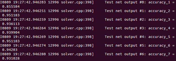
可看到第一个字符的识别率较为低,只有85%左右,其余的均在93%以上
五、使用训练得的模型做预测:
由于这里用的是python 接口,故先将之前的均值文件Mean.binaryproto 转为 mean.npy ,在Mean文件夹下新建 binToNpy.py ,使用以下代码转换
import numpy as np
import caffe
import sys

blob = caffe.proto.caffe_pb2.BlobProto()
data = open( 'mean.binaryproto' , 'rb' ).read()
blob.ParseFromString(data)
arr = np.array( caffe.io.blobproto_to_array(blob) )
out = arr[0]
np.save( 'mean.npy' , out )
这样deploy文件、均值文件、 caffemodel文件准备好了,在LPR下创建 predict.py ,载入一张图片作预测
#!/usr/bin/env python
#coding=utf-8

import cv2
import numpy as np
import sys,os
import time

import caffe

caffe_root = '/home/jyang/caffe/'
net_file = caffe_root + 'LPR/Proto/lpr_deploy.prototxt'
caffe_model = caffe_root + 'LPR/lpr_iter_40000.caffemodel'
mean_file = caffe_root + 'LPR/Mean/mean.npy'

img_path = caffe_root + 'LPR/001.png'    #图片路径

labels = {0 :"京", 1 :"沪", 2 :"津", 3 :"渝",4 : "冀" , 5: "晋",6: "蒙", 7: "辽",8: "吉",9: "黑",10: "苏",11: "浙",12: "皖",13:
         "闽",14: "赣",15: "鲁",16: "豫",17: "鄂",18: "湘",19: "粤",20: "桂",   21: "琼",22: "川",23: "贵",24: "云",
       25:  "藏",26: "陕",27: "甘",28: "青",29: "宁",30: "新",31: "0",32: "1",33: "2",34: "3",35: "4",36: "5",
       37:  "6",38: "7",39: "8",40: "9",41: "A",42: "B",43: "C",44: "D",45: "E",46: "F",47: "G",48: "H",
        49: "J",50: "K",51: "L",52: "M",53: "N",54: "P",55: "Q",56: "R",57: "S",58: "T",59: "U",60: "V",
        61: "W",62: "X",63: "Y",64: "Z" };

if __name__=='__main__':
    net=caffe.Net(net_file,caffe_model,caffe.TEST)
    transformer=caffe.io.Transformer({'data':net.blobs['data'].data.shape})
    transformer.set_transpose('data' ,(2, 0, 1) )
    #读入的是H*W*C(0,1,2),但我们需要的是C*H*W(2,0,1 )
    transformer.set_mean('data', np.load(mean_file).mean(1).mean(1) )
    transformer.set_raw_scale('data' , 255)
    #把数据从[0-1] rescale 至 [0-255]
    transformer.set_channel_swap('data' ,(2 ,1 , 0))
    #在caffe中读入是BGR(0,1,2),所以要将RGB转化为BGR(2,1,0)

    start = time.time()
    img=caffe.io.load_image(img_path )
    img=img[...,::-1]

    net.blobs['data'].data[...]=transformer.preprocess('data' , img)
    out=net.forward()

    prob=('prob_1','prob_2','prob_3','prob_4','prob_5','prob_6','prob_7')
    for k in range(7):
       index = net.blobs[prob[k]].data[0].flatten().argsort()[-1:-6:-1]
       print labels[index[0]],
    print("\nDone in %.2f s." % (time.time()-start ))

    cv2.imshow( 'demo',img)
    cv2.waitKey(0)


结语
实际测试图片,发现完全正确识别的准确率很低,虽然训练得到的模型在验证集上的识别准确率很高,但是训练集和验证集都是经过样本增强得到的,3922张扩充至80000多张,扩充的样本和真实样本还是存在差距,且即是扩充再多,样本信息还是有限的,导致过拟和了,如果能获得几万张真实的车牌图片,所训练出的模型实用性将会更高。


 348
348

 被折叠的 条评论
为什么被折叠?
被折叠的 条评论
为什么被折叠?
 到【灌水乐园】发言


