Node Classification with Graph Neural Networks(使用GNN进行节点分类）

各种机器学习应用中的许多数据集在其实体之间具有结构关系，可以表示为图。 比如社交和通信网络分析、流量预测和欺诈检测等。 图表示学习旨在为用于各种 ML 任务的图数据集构建和训练模型。
该 example演示了 图神经网络 (GNN)模型的简单实现。 该模型在 Cora 数据集上进行节点预测任务，以根据其单词和引文网络预测论文主题。
我们从头开始实现图卷积层，以更好地理解它们的工作原理。 但是，有许多基于 TensorFlow 的专门库提供了丰富的 GNN API，例如 Spectral、StellarGraph 和 GraphNets。

Setup

import os
import pandas as pd
import numpy as np
import networkx as nx
import matplotlib.pyplot as plt
import tensorflow as tf
from tensorflow import keras
from tensorflow.keras import layers

准备数据集

使用Cora dataset，该数据集包括2708科学文章，并且分类为七类。citation network 有5429个links（链接）。每篇论文有一个大小为1433的二进制词向量，表示相对应的词。
该数据集有两个文件：cora.cites和cora.content。

• cora.cites包括两列（cited_paper_id(target)和citing_paper_id(source)
• cora.content包括1435列的paper content records：paper_id,subject和1433二进制特征

下载数据集:

zip_file = keras.utils.get_file(
    fname="cora.tgz",
    origin="https://linqs-data.soe.ucsc.edu/public/lbc/cora.tgz",
    extract=True,
)
data_dir = os.path.join(os.path.dirname(zip_file), "cora")

运行如下：

处理和可视化数据集

加载citations data 到Pandas DataFrame中。

citations = pd.read_csv(
    os.path.join(data_dir, "cora.cites"),
    sep="\t",
    header=None,
    names=["target", "source"],
)
# print("Citations shape:", citations.shape) #(5429,2)

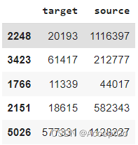
Display a sample of the citations DataFrame. The target 列包括paper ids cited by the paper ids 在source列。

citations.sample(frac=1).head()

然后加载paper data到Pandas DataFrame。

column_names = ["paper_id"] + [f"term_{idx}" for idx in range(1433)] + ["subject"]
papers = pd.read_csv(
    os.path.join(data_dir, "cora.content"), sep="\t", header=None, names=column_names,
)
print("Papers shape:", papers.shape) # (2708, 1435)

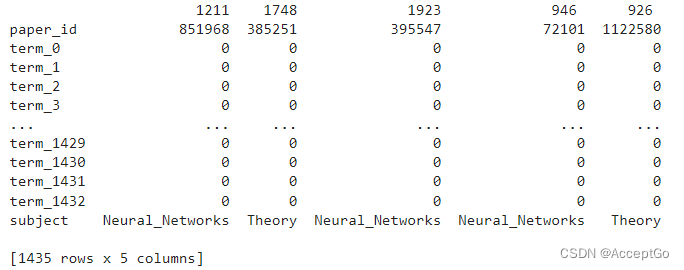
Display a sample of papers DataFrame. 该数据框包括paper_id和subject列以及1433二进制列表示在paper中是否存在一个term.

print(papers.sample(5).T)

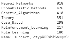
然后,展示每一个subject中paper的数量

print(papers.subject.value_counts())

然后，转换paper ids和subjects到zero-based indices.

class_values = sorted(papers["subject"].unique())
class_idx = {name: id for id, name in enumerate(class_values)}
paper_idx = {name: idx for idx, name in enumerate(sorted(papers["paper_id"].unique()))}

papers["paper_id"] = papers["paper_id"].apply(lambda name: paper_idx[name])
citations["source"] = citations["source"].apply(lambda name: paper_idx[name])
citations["target"] = citations["target"].apply(lambda name: paper_idx[name])
papers["subject"] = papers["subject"].apply(lambda value: class_idx[value])

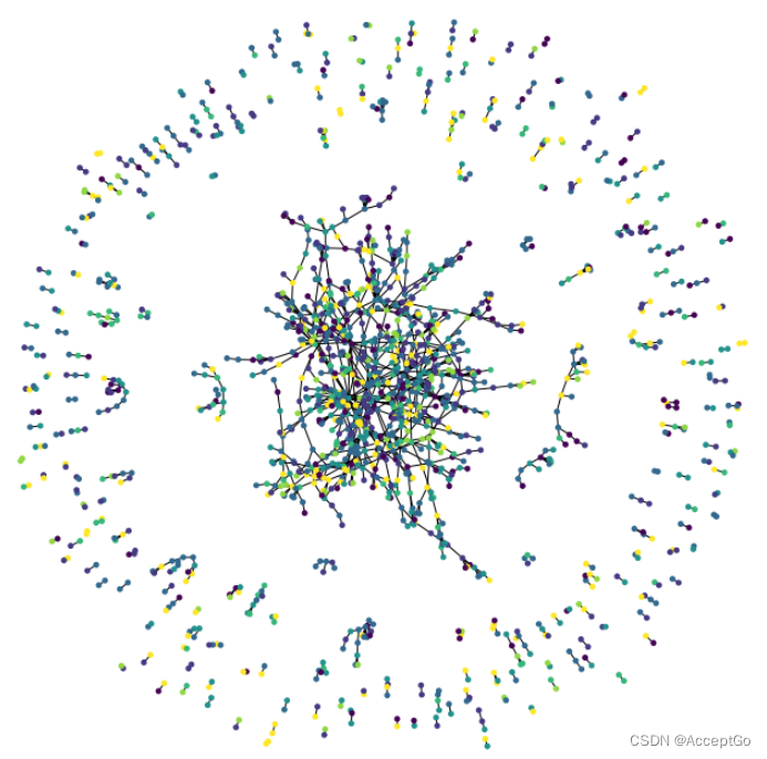
接着，可视化citation graph，图中的每个节点代表一篇paper，节点的颜色对应它的subject，下面展示的是数据集当中的一个sample。

plt.figure(figsize=(10, 10))
colors = papers["subject"].tolist()
cora_graph = nx.from_pandas_edgelist(citations.sample(n=1500))
subjects = list(papers[papers["paper_id"].isin(list(cora_graph.nodes))]["subject"])
nx.draw_spring(cora_graph, node_size=15, node_color=subjects)

拆分数据集为分层训练集和测试集

train_data, test_data = [], []

for _, group_data in papers.groupby("subject"):
    # Select around 50% of the dataset for training.
    random_selection = np.random.rand(len(group_data.index)) <= 0.5
    train_data.append(group_data[random_selection])
    test_data.append(group_data[~random_selection])

train_data = pd.concat(train_data).sample(frac=1)
test_data = pd.concat(test_data).sample(frac=1)

print("Train data shape:", train_data.shape) # (1335, 1435)
print("Test data shape:", test_data.shape) # (1373, 1435)

训练和评估的实现

hidden_units = [32, 32]
learning_rate = 0.01
dropout_rate = 0.5
num_epochs = 300
batch_size = 256

使用给定的数据训练输入模型

def run_experiment(model, x_train, y_train):
    # Compile the model.
    model.compile(
        optimizer=keras.optimizers.Adam(learning_rate),
        loss=keras.losses.SparseCategoricalCrossentropy(from_logits=True),
        metrics=[keras.metrics.SparseCategoricalAccuracy(name="acc")],
    )
    # Create an early stopping callback.
    early_stopping = keras.callbacks.EarlyStopping(
        monitor="val_acc", patience=50, restore_best_weights=True
    )
    # Fit the model.
    history = model.fit(
        x=x_train,
        y=y_train,
        epochs=num_epochs,
        batch_size=batch_size,
        validation_split=0.15,
        callbacks=[early_stopping],
    )

    return history

在训练期间展示模型的loss和accuracy

def display_learning_curves(history):
    fig, (ax1, ax2) = plt.subplots(1, 2, figsize=(15, 5))

    ax1.plot(history.history["loss"])
    ax1.plot(history.history["val_loss"])
    ax1.legend(["train", "test"], loc="upper right")
    ax1.set_xlabel("Epochs")
    ax1.set_ylabel("Loss")

    ax2.plot(history.history["acc"])
    ax2.plot(history.history["val_acc"])
    ax2.legend(["train", "test"], loc="upper right")
    ax2.set_xlabel("Epochs")
    ax2.set_ylabel("Accuracy")
    plt.show()

Feedforward Network（FFN）

baseline和GNN model中将使用这个模块

def create_ffn(hidden_units, dropout_rate, name=None):
    fnn_layers = []

    for units in hidden_units:
        fnn_layers.append(layers.BatchNormalization())
        fnn_layers.append(layers.Dropout(dropout_rate))
        fnn_layers.append(layers.Dense(units, activation=tf.nn.gelu))

    return keras.Sequential(fnn_layers, name=name)

构建一个Baseline神经网络模型

为baseline模型准备数据

feature_names = set(papers.columns) - {"paper_id", "subject"}
num_features = len(feature_names)
num_classes = len(class_idx)

# Create train and test features as a numpy array.
x_train = train_data[feature_names].to_numpy()
x_test = test_data[feature_names].to_numpy()
# Create train and test targets as a numpy array.
y_train = train_data["subject"]
y_test = test_data["subject"]

baseline classifier的实现
添加五个带有跳跃连接的FFN块，以便生成的baseline模型其参数数量和GNN模型大致相同。

def create_baseline_model(hidden_units, num_classes, dropout_rate=0.2):
    inputs = layers.Input(shape=(num_features,), name="input_features")
    x = create_ffn(hidden_units, dropout_rate, name=f"ffn_block1")(inputs)
    for block_idx in range(4):
        # Create an FFN block.
        x1 = create_ffn(hidden_units, dropout_rate, name=f"ffn_block{block_idx + 2}")(x)
        # Add skip connection.
        x = layers.Add(name=f"skip_connection{block_idx + 2}")([x, x1])
    # Compute logits.
    logits = layers.Dense(num_classes, name="logits")(x)
    # Create the model.
    return keras.Model(inputs=inputs, outputs=logits, name="baseline")

baseline_model = create_baseline_model(hidden_units, num_classes, dropout_rate)
baseline_model.summary()

训练baseline classifier

history = run_experiment(baseline_model, x_train, y_train)

画出学习曲线

display_learning_curves(history)

在测试集上评估baseline模型

_, test_accuracy = baseline_model.evaluate(x=x_test, y=y_test, verbose=0)
print(f"Test accuracy: {round(test_accuracy * 100, 2)}%")  # 72.25%

检查baseline模型预测

通过随机生成关于单词存在概率的二进制单词向量来创建新的数据实例。

def generate_random_instances(num_instances):
    token_probability = x_train.mean(axis=0)
    instances = []
    for _ in range(num_instances):
        probabilities = np.random.uniform(size=len(token_probability))
        instance = (probabilities <= token_probability).astype(int)
        instances.append(instance)

    return np.array(instances)


def display_class_probabilities(probabilities):
    for instance_idx, probs in enumerate(probabilities):
        print(f"Instance {instance_idx + 1}:")
        for class_idx, prob in enumerate(probs):
            print(f"- {class_values[class_idx]}: {round(prob * 100, 2)}%")

给定随机生成的实例，baseline 模型预测如下：

new_instances = generate_random_instances(num_classes)
logits = baseline_model.predict(new_instances)
probabilities = keras.activations.softmax(tf.convert_to_tensor(logits)).numpy()
display_class_probabilities(probabilities)

构建图神经网络模型

为图模型准备数据

准备图数据并将其加载到模型中进行训练是 GNN 模型中最具挑战性的部分，专门的库以不同的方式解决了这一问题。 在此示例中，展示了一种用于准备和使用图形数据的简单方法，该方法适用于数据集由一个完全适合内存的图形组成的情况

图数据由graph_info元组组成，包含以下三个元素：

• node_features：这是一个[num_nodes,num_features] Numpy 数组，其包括节点特征，该数据集中，nodes是papers，node_features是每篇paper的word-presence 二进制向量。
• edges：[num_edges,num_edges] Numpy数组表示两个nodes之间的links的稀疏邻接矩阵。该例中，links是citations和papers的关联。
• edge_weights（可选）：[num_edges] Numpy数组，包括边的权重，衡量图中节点的关系，该例中，paper citations没有权重。
• Update：The node_repesentations and aggregated_messages—both of shape [num_nodes, representation_dim]— are combined and processed to produce the new state of the node representations (node embeddings). If combination_type is gru, the node_repesentations and aggregated_messages are stacked to create a sequence, then processed by a GRU layer. Otherwise, the node_repesentations and aggregated_messages are added or concatenated, then processed using a FFN.
  The technique implemented use ideas from Graph Convolutional Networks, GraphSage, Graph Isomorphism Network, Simple Graph Networks, and Gated Graph Sequence Neural Networks. Two other key techniques that are not covered are Graph Attention Networks and Message Passing Neural Networks.

# Create an edges array (sparse adjacency matrix) of shape [2, num_edges].
edges = citations[["source", "target"]].to_numpy().T
# Create an edge weights array of ones.
edge_weights = tf.ones(shape=edges.shape[1])
# Create a node features array of shape [num_nodes, num_features].
node_features = tf.cast(
    papers.sort_values("paper_id")[feature_names].to_numpy(), dtype=tf.dtypes.float32
)
# Create graph info tuple with node_features, edges, and edge_weights.
graph_info = (node_features, edges, edge_weights)

print("Edges shape:", edges.shape)  #  (2, 5429)
print("Nodes shape:", node_features.shape) # (2708, 1433)

图卷积层的实现

下面实现一个图卷积模块作为一个Keras Layer，步骤如下：

• Prepare：输入节点表示使用FFN处理产生一个消息。可以仅通过线性变换来简化表示。
• Aggregate：每个节点的邻接点消息通过使用permutation invariant pooling 操作关于edge_weights进行聚合，比如sum、mean、max为每个节点准备一条聚合消息。比如，math.unsorted_segment_sum 用来聚合neighbour消息.

class GraphConvLayer(layers.Layer):
    def __init__(
        self,
        hidden_units,
        dropout_rate=0.2,
        aggregation_type="mean",
        combination_type="concat",
        normalize=False,
        *args,
        **kwargs,
    ):
        super(GraphConvLayer, self).__init__(*args, **kwargs)

        self.aggregation_type = aggregation_type
        self.combination_type = combination_type
        self.normalize = normalize

        self.ffn_prepare = create_ffn(hidden_units, dropout_rate)
        if self.combination_type == "gated":
            self.update_fn = layers.GRU(
                units=hidden_units,
                activation="tanh",
                recurrent_activation="sigmoid",
                dropout=dropout_rate,
                return_state=True,
                recurrent_dropout=dropout_rate,
            )
        else:
            self.update_fn = create_ffn(hidden_units, dropout_rate)

    def prepare(self, node_repesentations, weights=None):
        # node_repesentations shape is [num_edges, embedding_dim].
        messages = self.ffn_prepare(node_repesentations)
        if weights is not None:
            messages = messages * tf.expand_dims(weights, -1)
        return messages

    def aggregate(self, node_indices, neighbour_messages):
        # node_indices shape is [num_edges].
        # neighbour_messages shape: [num_edges, representation_dim].
        num_nodes = tf.math.reduce_max(node_indices) + 1
        if self.aggregation_type == "sum":
            aggregated_message = tf.math.unsorted_segment_sum(
                neighbour_messages, node_indices, num_segments=num_nodes
            )
        elif self.aggregation_type == "mean":
            aggregated_message = tf.math.unsorted_segment_mean(
                neighbour_messages, node_indices, num_segments=num_nodes
            )
        elif self.aggregation_type == "max":
            aggregated_message = tf.math.unsorted_segment_max(
                neighbour_messages, node_indices, num_segments=num_nodes
            )
        else:
            raise ValueError(f"Invalid aggregation type: {self.aggregation_type}.")

        return aggregated_message

    def update(self, node_repesentations, aggregated_messages):
        # node_repesentations shape is [num_nodes, representation_dim].
        # aggregated_messages shape is [num_nodes, representation_dim].
        if self.combination_type == "gru":
            # Create a sequence of two elements for the GRU layer.
            h = tf.stack([node_repesentations, aggregated_messages], axis=1)
        elif self.combination_type == "concat":
            # Concatenate the node_repesentations and aggregated_messages.
            h = tf.concat([node_repesentations, aggregated_messages], axis=1)
        elif self.combination_type == "add":
            # Add node_repesentations and aggregated_messages.
            h = node_repesentations + aggregated_messages
        else:
            raise ValueError(f"Invalid combination type: {self.combination_type}.")

        # Apply the processing function.
        node_embeddings = self.update_fn(h)
        if self.combination_type == "gru":
            node_embeddings = tf.unstack(node_embeddings, axis=1)[-1]

        if self.normalize:
            node_embeddings = tf.nn.l2_normalize(node_embeddings, axis=-1)
        return node_embeddings

    def call(self, inputs):
        """Process the inputs to produce the node_embeddings.

        inputs: a tuple of three elements: node_repesentations, edges, edge_weights.
        Returns: node_embeddings of shape [num_nodes, representation_dim].
        """

        node_repesentations, edges, edge_weights = inputs
        # Get node_indices (source) and neighbour_indices (target) from edges.
        node_indices, neighbour_indices = edges[0], edges[1]
        # neighbour_repesentations shape is [num_edges, representation_dim].
        neighbour_repesentations = tf.gather(node_repesentations, neighbour_indices)

        # Prepare the messages of the neighbours.
        neighbour_messages = self.prepare(neighbour_repesentations, edge_weights)
        # Aggregate the neighbour messages.
        aggregated_messages = self.aggregate(node_indices, neighbour_messages)
        # Update the node embedding with the neighbour messages.
        return self.update(node_repesentations, aggregated_messages)

图神经网络节点分类

GNN 分类模型遵循Design Space for Graph Neural Networks 方法，如下：

• 使用FFN对节点特征进行预处理生成初始化节点表示
• 将一个多多个带有跳跃连接的图卷积层应用于节点表示生成节点嵌入
• 使用FFN对节点嵌入应用后处理以生成最终节点嵌入
• 在 Softmax 层中输入节点嵌入以预测节点类别。
  添加的每个图卷积层都从更高级别的邻居捕获信息。 但是，添加许多图卷积层会导致过度平滑，其中模型会为所有节点生成相似的嵌入

请注意，graph_info 传递给 Keras 模型的构造函数，并用作 Keras 模型对象的属性，而不是用于训练或预测的输入数据。 该模型将接受一批 node_indices，用于从 graph_info 中查找节点特征和邻居。

class GNNNodeClassifier(tf.keras.Model):
    def __init__(
        self,
        graph_info,
        num_classes,
        hidden_units,
        aggregation_type="sum",
        combination_type="concat",
        dropout_rate=0.2,
        normalize=True,
        *args,
        **kwargs,
    ):
        super(GNNNodeClassifier, self).__init__(*args, **kwargs)

        # Unpack graph_info to three elements: node_features, edges, and edge_weight.
        node_features, edges, edge_weights = graph_info
        self.node_features = node_features
        self.edges = edges
        self.edge_weights = edge_weights
        # Set edge_weights to ones if not provided.
        if self.edge_weights is None:
            self.edge_weights = tf.ones(shape=edges.shape[1])
        # Scale edge_weights to sum to 1.
        self.edge_weights = self.edge_weights / tf.math.reduce_sum(self.edge_weights)

        # Create a process layer.
        self.preprocess = create_ffn(hidden_units, dropout_rate, name="preprocess")
        # Create the first GraphConv layer.
        self.conv1 = GraphConvLayer(
            hidden_units,
            dropout_rate,
            aggregation_type,
            combination_type,
            normalize,
            name="graph_conv1",
        )
        # Create the second GraphConv layer.
        self.conv2 = GraphConvLayer(
            hidden_units,
            dropout_rate,
            aggregation_type,
            combination_type,
            normalize,
            name="graph_conv2",
        )
        # Create a postprocess layer.
        self.postprocess = create_ffn(hidden_units, dropout_rate, name="postprocess")
        # Create a compute logits layer.
        self.compute_logits = layers.Dense(units=num_classes, name="logits")

    def call(self, input_node_indices):
        # Preprocess the node_features to produce node representations.
        x = self.preprocess(self.node_features)
        # Apply the first graph conv layer.
        x1 = self.conv1((x, self.edges, self.edge_weights))
        # Skip connection.
        x = x1 + x
        # Apply the second graph conv layer.
        x2 = self.conv2((x, self.edges, self.edge_weights))
        # Skip connection.
        x = x2 + x
        # Postprocess node embedding.
        x = self.postprocess(x)
        # Fetch node embeddings for the input node_indices.
        node_embeddings = tf.gather(x, input_node_indices)
        # Compute logits
        return self.compute_logits(node_embeddings)

测试初始化，并调用GNN模型，若提供了N个节点索引，不论图的大小是多少，输出的tensor形状都是[N,num_classes]。

gnn_model = GNNNodeClassifier(
    graph_info=graph_info,
    num_classes=num_classes,
    hidden_units=hidden_units,
    dropout_rate=dropout_rate,
    name="gnn_model",
)

print("GNN output shape:", gnn_model([1, 10, 100]))

gnn_model.summary()

训练GNN模型

使用标准的监督cross-entropy loss训练模型，然而，可以为生成的节点嵌入添加另一个自监督损失项，确保图中邻居节点有相似的表示，而远处的节点有不同的表示。

x_train = train_data.paper_id.to_numpy()
history = run_experiment(gnn_model, x_train, y_train)

画出学习曲线如下：

display_learning_curves(history)

现在在测试集上评估GNN模型，结果可能因训练样本而异，但GNN模型在test accuracy上总是优于baseline模型。

x_test = test_data.paper_id.to_numpy()
_, test_accuracy = gnn_model.evaluate(x=x_test, y=y_test, verbose=0)
print(f"Test accuracy: {round(test_accuracy * 100, 2)}%")  # 77.49%

GNN模型预测

添加新的实例作为nodes到node_features，并和已经存在的nodes生成links(citations)。

# First we add the N new_instances as nodes to the graph
# by appending the new_instance to node_features.
num_nodes = node_features.shape[0]
new_node_features = np.concatenate([node_features, new_instances])
# Second we add the M edges (citations) from each new node to a set
# of existing nodes in a particular subject
new_node_indices = [i + num_nodes for i in range(num_classes)]
new_citations = []
for subject_idx, group in papers.groupby("subject"):
    subject_papers = list(group.paper_id)
    # Select random x papers specific subject.
    selected_paper_indices1 = np.random.choice(subject_papers, 5)
    # Select random y papers from any subject (where y < x).
    selected_paper_indices2 = np.random.choice(list(papers.paper_id), 2)
    # Merge the selected paper indices.
    selected_paper_indices = np.concatenate(
        [selected_paper_indices1, selected_paper_indices2], axis=0
    )
    # Create edges between a citing paper idx and the selected cited papers.
    citing_paper_indx = new_node_indices[subject_idx]
    for cited_paper_idx in selected_paper_indices:
        new_citations.append([citing_paper_indx, cited_paper_idx])

new_citations = np.array(new_citations).T
new_edges = np.concatenate([edges, new_citations], axis=1)

更新GNN模型中的node_features和edges

print("Original node_features shape:", gnn_model.node_features.shape)
print("Original edges shape:", gnn_model.edges.shape)
gnn_model.node_features = new_node_features
gnn_model.edges = new_edges
gnn_model.edge_weights = tf.ones(shape=new_edges.shape[1])
print("New node_features shape:", gnn_model.node_features.shape)
print("New edges shape:", gnn_model.edges.shape)

logits = gnn_model.predict(tf.convert_to_tensor(new_node_indices))
probabilities = keras.activations.softmax(tf.convert_to_tensor(logits)).numpy()
display_class_probabilities(probabilities)

可以看到，同baseline模型相比，expected subjects的概率更高。