


本文首发于公众号:医学和生信笔记
“医学和生信笔记,专注R语言在临床医学中的使用,R语言数据分析和可视化。主要分享R语言做医学统计学、meta分析、网络药理学、临床预测模型、机器学习、生物信息学等。
C-statistic是评价模型区分度的指标之一,在logistic模型中,C-statistic就是AUC,在生存资料中,C-statistic和AUC略有不同。
今天给大家分别介绍logistic和cox回归的C-statistic计算方法。
logistic回归的C-statistic
今天学习C-index的4种计算方法,在二分类变量中,C-statistic就是AUC,二者在数值上是一样的。
使用lowbirth数据集,这个数据集是关于低出生体重儿是否会死亡的数据集,其中dead这一列是结果变量,0代表死亡,1代表存活,其余列都是预测变量。数据的预处理和之前一样。
lowbirth <- read.csv("../000files/lowbirth.csv")

library(dplyr)
## Warning: 程辑包'dplyr'是用R版本4.1.2 来建造的
##
## 载入程辑包:'dplyr'
## The following objects are masked from 'package:stats':
##
##     filter, lag
## The following objects are masked from 'package:base':
##
##     intersect, setdiff, setequal, union

tmp <- lowbirth %>%
  mutate(across(where(is.character),as.factor),
         vent = factor(vent),
         black = ifelse(race == "black",1,0),
         white = ifelse(race == "white",1,0),
         other = ifelse(race %in% c("native American","oriental"),1,0)
         ) %>%
  select(- race)

glimpse(tmp)
## Rows: 565
## Columns: 12
## $ birth    <dbl> 81.514, 81.552, 81.558, 81.593, 81.610, 81.624, 81.626, 81.68~
## $ lowph    <dbl> 7.250000, 7.059998, 7.250000, 6.969997, 7.320000, 7.160000, 7~
## $ pltct    <int> 244, 114, 182, 54, 282, 153, 229, 182, 361, 378, 255, 186, 26~
## $ bwt      <int> 1370, 620, 1480, 925, 1255, 1350, 1310, 1110, 1180, 970, 770,~
## $ delivery <fct> abdominal, vaginal, vaginal, abdominal, vaginal, abdominal, v~
## $ apg1     <int> 7, 1, 8, 5, 9, 4, 6, 6, 6, 2, 4, 8, 1, 8, 5, 9, 9, 9, 6, 2, 1~
## $ vent     <fct> 0, 1, 0, 1, 0, 0, 1, 0, 0, 1, 1, 0, 1, 1, 0, 1, 0, 0, 1, 0, 1~
## $ sex      <fct> female, female, male, female, female, female, male, male, mal~
## $ dead     <int> 0, 1, 0, 1, 0, 0, 0, 0, 0, 1, 0, 0, 0, 0, 0, 0, 0, 0, 1, 0, 0~
## $ black    <dbl> 0, 1, 1, 1, 1, 1, 0, 1, 0, 0, 1, 0, 1, 0, 0, 1, 0, 1, 1, 1, 0~
## $ white    <dbl> 1, 0, 0, 0, 0, 0, 1, 0, 1, 1, 0, 1, 0, 1, 1, 0, 1, 0, 0, 0, 1~
## $ other    <dbl> 0, 0, 0, 0, 0, 0, 0, 0, 0, 0, 0, 0, 0, 0, 0, 0, 0, 0, 0, 0, 0~
方法1
使用rms包构建模型,模型结果中Rank Discrim.下面的C 就是C-Statistic,本模型中C-Statistic = 0.879。
library(rms)
## 载入需要的程辑包:Hmisc
## 载入需要的程辑包:lattice
## 载入需要的程辑包:survival
## 载入需要的程辑包:Formula
## 载入需要的程辑包:ggplot2
## Warning: 程辑包'ggplot2'是用R版本4.1.3 来建造的
##
## 载入程辑包:'Hmisc'
## The following objects are masked from 'package:dplyr':
##
##     src, summarize
## The following objects are masked from 'package:base':
##
##     format.pval, units
## 载入需要的程辑包:SparseM
##
## 载入程辑包:'SparseM'
## The following object is masked from 'package:base':
##
##     backsolve

fit2 <- lrm(dead ~ birth + lowph + pltct + bwt + vent + black + white,
            data = tmp,x=T,y=T)

fit2
## Logistic Regression Model
##
##  lrm(formula = dead ~ birth + lowph + pltct + bwt + vent + black +
##      white, data = tmp, x = T, y = T)
##
##                         Model Likelihood    Discrimination    Rank Discrim.
##                               Ratio Test           Indexes          Indexes
##  Obs           565    LR chi2     167.56    R2       0.432    C       0.879
##   0            471    d.f.             7    g        2.616    Dxy     0.759
##   1             94    Pr(> chi2) <0.0001    gr      13.682    gamma   0.759
##  max |deriv| 1e-06                          gp       0.210    tau-a   0.211
##                                             Brier    0.095
##
##            Coef    S.E.    Wald Z Pr(>|Z|)
##  Intercept 38.3815 11.0303  3.48  0.0005
##  birth     -0.1201  0.0914 -1.31  0.1890
##  lowph     -4.1451  1.1881 -3.49  0.0005
##  pltct     -0.0017  0.0019 -0.91  0.3644
##  bwt       -0.0031  0.0006 -5.14  <0.0001
##  vent=1     2.7526  0.7436  3.70  0.0002
##  black      1.1974  0.8448  1.42  0.1564
##  white      0.8597  0.8655  0.99  0.3206
##
方法2
ROCR包计算AUC,logistic回归的AUC就是C-statistic。这种方法和SPSS得到的一样。
library(ROCR)

tmp$predvalue<-predict(fit2)

# 取出C-Statistics,和上面结果一样
pred <- prediction(tmp$predvalue, tmp$dead)

auc <- round(performance(pred, "auc")@y.values[[1]],digits = 4)
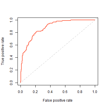
这个包也是用来画ROC曲线常用的包,可以根据上面的结果直接画出ROC曲线:
perf <- performance(pred,"tpr","fpr")
plot(perf,col="tomato",lwd=2)
abline(0,1,lty=2, col="grey")
方法3
pROC包计算AUC,这个包也是画ROC曲线常用的R包,但是这个包在使用时需要注意,下次再说。
library(pROC)
## Type 'citation("pROC")' for a citation.
##
## 载入程辑包:'pROC'
## The following objects are masked from 'package:stats':
##
##     cov, smooth, var

# 计算AUC,也就是C-statistic
roc(tmp$dead, tmp$predvalue, legacy.axes = T, print.auc = T, print.auc.y = 45)
## Setting levels: control = 0, case = 1
## Setting direction: controls < cases
##
## Call:
## roc.default(response = tmp$dead, predictor = tmp$predvalue, legacy.axes = T,     print.auc = T, print.auc.y = 45)
##
## Data: tmp$predvalue in 471 controls (tmp$dead 0) < 94 cases (tmp$dead 1).
## Area under the curve: 0.8794
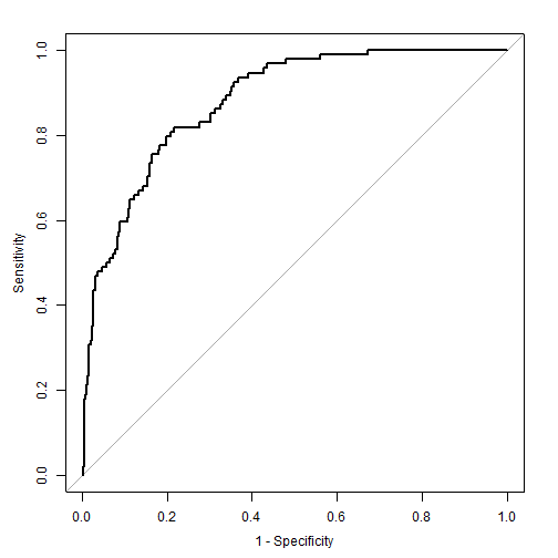
也是可以直接画法ROC曲线的:
roc.plot <- roc(tmp$dead, tmp$predvalue)
## Setting levels: control = 0, case = 1
## Setting direction: controls < cases
plot(roc.plot,legacy.axes=T)
方法4
使用Hmisc包。结果中的C就是C-Statistic。
library(Hmisc)
somers2(tmp$predvalue, tmp$dead)
##           C         Dxy           n     Missing
##   0.8793875   0.7587749 565.0000000   0.0000000
cox回归的C-statistic
cox回归的C-statistic可以用survival包计算,需要注意,生存分析的C-statistic和AUC是不一样的。
使用survival包自带的lung数据集进行演示。
library(survival)
library(dplyr)

df1 <- lung %>%
  mutate(status=ifelse(status == 1,1,0))

str(lung)
## 'data.frame': 228 obs. of  10 variables:
##  $ inst     : num  3 3 3 5 1 12 7 11 1 7 ...
##  $ time     : num  306 455 1010 210 883 ...
##  $ status   : num  2 2 1 2 2 1 2 2 2 2 ...
##  $ age      : num  74 68 56 57 60 74 68 71 53 61 ...
##  $ sex      : num  1 1 1 1 1 1 2 2 1 1 ...
##  $ ph.ecog  : num  1 0 0 1 0 1 2 2 1 2 ...
##  $ ph.karno : num  90 90 90 90 100 50 70 60 70 70 ...
##  $ pat.karno: num  100 90 90 60 90 80 60 80 80 70 ...
##  $ meal.cal : num  1175 1225 NA 1150 NA ...
##  $ wt.loss  : num  NA 15 15 11 0 0 10 1 16 34 ...
cox_fit1 <- coxph(Surv(time, status) ~ age + sex + ph.ecog + ph.karno + pat.karno,
              data = lung,x = T, y = T)

summary(cox_fit1)
## Call:
## coxph(formula = Surv(time, status) ~ age + sex + ph.ecog + ph.karno +
##     pat.karno, data = lung, x = T, y = T)
##
##   n= 223, number of events= 160
##    (因为不存在,5个观察量被删除了)
##
##                coef exp(coef)  se(coef)      z Pr(>|z|)
## age        0.011383  1.011448  0.009510  1.197  0.23134
## sex       -0.561464  0.570373  0.170689 -3.289  0.00100 **
## ph.ecog    0.565533  1.760386  0.186716  3.029  0.00245 **
## ph.karno   0.015853  1.015979  0.009853  1.609  0.10762
## pat.karno -0.010111  0.989940  0.006881 -1.470  0.14169
## ---
## Signif. codes:  0 '***' 0.001 '**' 0.01 '*' 0.05 '.' 0.1 ' ' 1
##
##           exp(coef) exp(-coef) lower .95 upper .95
## age          1.0114     0.9887    0.9928     1.030
## sex          0.5704     1.7532    0.4082     0.797
## ph.ecog      1.7604     0.5681    1.2209     2.538
## ph.karno     1.0160     0.9843    0.9965     1.036
## pat.karno    0.9899     1.0102    0.9767     1.003
##
## Concordance= 0.647  (se = 0.025 )
## Likelihood ratio test= 32.9  on 5 df,   p=4e-06
## Wald test            = 33  on 5 df,   p=4e-06
## Score (logrank) test = 33.79  on 5 df,   p=3e-06
Concordance就是C-statistic,本次示例中为0.647。
以上就是C-statistic的计算。
获取lowbirth数据请在公众号后台回复20220520
本文首发于公众号:医学和生信笔记
“医学和生信笔记,专注R语言在临床医学中的使用,R语言数据分析和可视化。主要分享R语言做医学统计学、meta分析、网络药理学、临床预测模型、机器学习、生物信息学等。
本文由 mdnice 多平台发布


 5181
5181


 被折叠的 条评论
为什么被折叠?
被折叠的 条评论
为什么被折叠?
 到【灌水乐园】发言


