


 本文围绕SAC框架学习展开,结合倒立摆问题,总结学习收获与思考。介绍强化学习与机器学习联系、深度强化学习结合领域及常见方法。详细解释代码各部分,包括调包、环境初始化、网络结构设计、训练策略、参数更新等,还给出可运行代码及结果。
文章目录
概要
本文主要通过倒立摆的问题,总结本人在SAC框架学习过程的收获和思考。为使得学习有效,对于代码的框架和细节处会多加注释,确认理解了框架和细节,使其具有一定的迁移能力。
前部分的总结是按照学习的文章的作者的思考逻辑总结的,实际运行代码的顺序在最后。
以下是学习的参考:
https://towardsdatascience.com/soft-actor-critic-demystified-b8427df61665(理论部分)
https://github.com/vaishak2future/sac/blob/master/sac.ipynb(Github代码部分)
https://github.com/higgsfield/RL-Adventure-2(Github本文分析的代码部分的参照代码)
部分文案使用ChatGPT4补充。
本人也在学习探索中,内容仅供参考,如有错误请多多指正。
背景知识调研及延伸
强化学习和机器学习的联系
强化学习 (RL) 强化学习是机器学习的一个子领域,用于解决决策过程问题,例如游戏、机器人导航、资源管理等。RL基于奖励系统来进行学习:对于给定的状态,代理(agent)会执行一个动作,并从环境中接收一个反馈(奖励或惩罚)。RL的目标是找到一个策略,使得代理能够通过执行一系列的动作来最大化累积奖励。
强化学习的可能结合领域(Deep Reinforcement Learning,DRL)
卷积神经网络(Convolutional Neural Networks,CNN)和强化学习(Reinforcement Learning,RL)是两种在人工智能领域中不同的机器学习方法。但是这两者其实可以结合使用。思路如下:
卷积神经网络 (CNN) CNN是一种深度学习的技术,主要用于处理具有网格结构的数据,例如图像(2D网格像素)和音频(1D网格)。CNN的特点在于其卷积层,通过滑动窗口(或卷积核)在输入数据上移动并执行卷积运算,从而可以在保留空间结构信息的同时,有效地学习局部特征。CNN还包括池化层(用于进行降采样)和全连接层(进行分类或回归)。
在强化学习的环境中,可以使用CNN来处理视觉输入,然后根据CNN提取的特征来选择动作。这就是深度强化学习(Deep Reinforcement Learning,DRL)的基本思想。
常见的深度强化学习方法总结
- Monte-Carlo Methods(蒙特卡洛方法)
- Temporal Difference Methods and Q-learning(时间差分方法和Q学习)
- Deep Q-Network (DQN) for Reinforcement Learning in Continuous Space(连续空间强化学习的深度Q网络
- Function Approximation and Neural Network(函数逼近和神经网络)
- Policy-Based Methods, Hill-Climbing, Simulated Annealing(基于策略的方法,爬山算法,模拟退火)
- Policy-Gradient Methods, REINFORCE, Proximal Policy Optimization
(PPO)(基于策略梯度的方法,REINFORCE,近端策略优化) - Actor-Critic Methods, Asynchronous,Advantage Actor-Critic (A3C), Advantage Actor-Critic (A2C), DeepDeterministic Policy Gradient (DDPG), Twin Delayed DDPG (TD3), Soft
Actor-Critic
(SAC)(演员-评论家方法,异步优势演员-评论家,优势演员-评论家,深度确定性策略梯度,双延迟DDPG,软演员-评论家)
代码解释
提示:这里可以添加技术细节
Part1. 调包的部分,数据处理,使用现成的torch框架下的结构,图像处理部分,绘图等等
 import math
import random
import gym
import numpy as np

import torch
import torch.nn as nn
import torch.optim as optim
import torch.nn.functional as F
from torch.distributions import Normal

from IPython.display import clear_output
import matplotlib.pyplot as plt
from matplotlib import animation
from IPython.display import display

%matplotlib inline
Part2.确认是否有GPU,确认使用CPU还是GPU
use_cuda = torch.cuda.is_available()
device   = torch.device("cuda" if use_cuda else "cpu")
Part3.结构构建第一步,初始化环境,设计网络结构
从整体框架的角度理解,
1.确认我们要进行强化学习游戏时所处的环境,储存我们需要的观测维度参数。
储存关于环境观测维度(即状态,state),动作空间维度的信息(即动作,action)。即强化学习中两个重要的概念:状态,动作。 还有超参数,比如hidden layer的层数。
- 初始化我们的网络
初始化网络在我的理解中是设计完网络后,实例化进行初始结构搭建。作者应该希望我们先理解框架,所以在文章中首先提到SAC的初始化结构。
因为使用SAC结构,所以,我们需要初始化四个网络。我是这样做分类的:训练过程中被使用的网络,和训练完后被使用的网络。
训练过程中被使用的网络,即在模型训练完成前,我们还要更新网络参数时所涉及的网络。其实,训练过程中四个网络都被使用了,他们的职能如下:
- 网络soft_q_net1 和 soft_q_net2两个soft Q network用以计算状态-动作对的值。使用soft_q_net1和soft_q_net2两个Q网络是为了进行双重学习(Double Learning),可以减少过度估计的影响,从而提高学习的稳定性。
- value_net用以估计每个状态的值,两个网络共同提高网络稳定性。
- policy_net为策略网络,输出在给定状态下的应采取的动作,形式为其概率分布。
训练完后被使用的网络,在结束训练后不再被使用的网络,target_value_net不会再被使用。
- target_value_net从value_net部分复制而来,但是权重更新频率会更低,这样可以在整个训练过程中提供一个相对稳定的目标值,让训练过程更加稳定。模型训练完成后,训练完成后,我们通常只会使用value_net来进行决策或验证性能。而target_value_net更多的是在训练过程中提供帮助,训练完成后,我们通常不再需要它。
从细节的角度考虑,这段代码有两个小点:
-
最开始的动作空间标准化。大白话就是将agent在不同的游戏中的执行动作统一到一个范围内,避免不同游戏中的动作幅度不一样对结果产生影响。
-
对于隐藏层的层数设置问题,是一个可调节的点,增加隐藏层的层数也可能增加模型的复杂性和训练难度。如果隐藏层的层数过多或过少,都可能导致模型过拟合或欠拟合的问题。
#initialize the environment
env = NormalizedActions(gym.make("Pendulum-v1"))

action_dim = env.action_space.shape[0] #the dimension of the action space
state_dim  = env.observation_space.shape[0] #dimension of the observations of the environment
hidden_dim = 256 # the hyperparameter of how many hidden layers we want in our networks

#We initialize the main and target V networks to have the same parameters.
value_net    = ValueNetwork(state_dim, hidden_dim).to(device)
target_value_net = ValueNetwork(state_dim, hidden_dim).to(device) #create a second network which lags the main network called the target network.

#maintain two Q networks to solve the problem of overestimation of Q-values
soft_q_net1 = SoftQNetwork(state_dim, action_dim, hidden_dim).to(device)
soft_q_net2 = SoftQNetwork(state_dim, action_dim, hidden_dim).to(device)

#policy updates
policy_net = PolicyNetwork(state_dim, action_dim, hidden_dim).to(device)

for target_param, param in zip(target_value_net.parameters(), value_net.parameters()):
    target_param.data.copy_(param.data)

value_criterion  = nn.MSELoss()
soft_q_criterion1 = nn.MSELoss()
soft_q_criterion2 = nn.MSELoss()

value_lr  = 3e-4
soft_q_lr = 3e-4
policy_lr = 3e-4

value_optimizer  = optim.Adam(value_net.parameters(), lr=value_lr)
soft_q_optimizer1 = optim.Adam(soft_q_net1.parameters(), lr=soft_q_lr)
soft_q_optimizer2 = optim.Adam(soft_q_net2.parameters(), lr=soft_q_lr)
policy_optimizer = optim.Adam(policy_net.parameters(), lr=policy_lr)


replay_buffer_size = 1000000
replay_buffer = ReplayBuffer(replay_buffer_size)
Part4 确认训练策略
在我的理解里,设计网络结构就是制造一个可以用来进行SAC训练的工具,制造完工具的下一步是执行。SAC的训练过程就是智能体学习,执行的过程。只要执行,就存在策略,因此设计策略将决定agent的探索方式。
以下代码中,可以看到的策略是,只有当智能体已经执行了超过1000步之后,才开始使用策略网络选择行动。这是一种常见的训练策略,通常在训练初期让智能体随机行动以进行探索,而在训练后期,当策略网络已经学到一些策略后,再使用策略网络进行决策。
#nested loops
#The outer loop initializes the environment for the beginning of the episode.
while frame_idx < max_frames:
    state = env.reset()
    episode_reward = 0

# Polyak averaging method
    for step in range(max_steps):
        if frame_idx >1000:
            action = policy_net.get_action(state).detach() #sample an action from the Policy network
            next_state, reward, done, _ = env.step(action.numpy())
        else:
            action = env.action_space.sample() #sample an action randomly from the action space for the first few time steps(1000)
            next_state, reward, done, _ = env.step(action)


        replay_buffer.push(state, action, reward, next_state, done)

        state = next_state
        episode_reward += reward
        frame_idx += 1

        if len(replay_buffer) > batch_size:
            update(batch_size)

        if frame_idx % 1000 == 0:
            plot(frame_idx, rewards)

        if done:
            break

    rewards.append(episode_reward)
Part5 神经网络参数更新过程
参数更新过程即训练的过程,使用我们刚才定义好的网络结构,确定我们的reward后,对目标进行Q网络,V网络,Policy网络的训练。接下来说一下不同网络的更新方式。
在理解不同网络的更新方式之前我们首先理解一下不同网络的作用。Q网络得到的Q值,是在给定策略下,选择特定行动的状态的预期回报。V网络的V值,是在给定策略下,不论选择哪个行动,状态的预期回报。V值预测偏整体,Q值预测偏个体。
因此,对于value network的更新思路如下:
- Q网络更新时,SAC算法的特性是使用两个Q网络,以此来减少过度估计以及提高训练的稳定性。
- V网络更新时,从新预测的Q值中去除整体影响,从预测的新Q值中减去对数概率,即减去Policy在状态下选择某个行动的对数概率,能够从新的预测的Q值中除掉这部分的影响。最终得到新的目标V值。
这里也有几个细节补充:
-
贝尔曼方程计算得到的Q训练网络的目标target_q_value,其使用了当前奖励(reward)和下一个状态的预期价值(target_value,通过V网络计算),乘以一个折扣因子gamma,表示未来回报相比即时回报有更小的价值。
-
target_value_func = predicted_new_q_value - log_prob的理解
目标值函数等于预测的新 Q 值减去选择新行动的对数概率。这是 Soft Actor-Critic(SAC)算法的一个关键部分,该算法通过最大化 Q 值和熵的期望和来改善策略。在这个公式中,log_prob 被减去是因为我们希望在选择行动时考虑到熵,增加策略的探索性,这是通过优化策略的熵来实现的,熵在这里被表示为负对数概率(因为对数概率通常是负数,所以减去对数概率就等于添加熵)。
3.policy_loss = (log_prob - predicted_new_q_value).mean()的理解
策略损失的计算是Soft Actor-Critic算法的关键部分,目的是最大化预期的奖励和熵的和。即最小化 policy_loss,即最小化 (log_prob - predicted_new_q_value)。(log_prob - predicted_new_q_value) 的作用是找到一个在最大化预期奖励和策略熵之间的平衡点。
有一个理解的细节是,在 Soft Actor-Critic(SAC)算法中,我们希望最大化策略的熵,这通常意味着我们希望最大化 log_prob 的绝对值(也就是让 log_prob 的值尽可能小)。这是因为,最大化熵就是要使策略更倾向于探索更多可能的行动,而这通常意味着选择那些对数概率(即 log_prob)的绝对值较大(值较小)的行动。
#network update

def update(batch_size,gamma=0.99,soft_tau=1e-2,):

    state, action, reward, next_state, done = replay_buffer.sample(batch_size)

    state      = torch.FloatTensor(state).to(device)
    next_state = torch.FloatTensor(next_state).to(device)
    action     = torch.FloatTensor(action).to(device)
    reward     = torch.FloatTensor(reward).unsqueeze(1).to(device)
    done       = torch.FloatTensor(np.float32(done)).unsqueeze(1).to(device)

    predicted_q_value1 = soft_q_net1(state, action)
    predicted_q_value2 = soft_q_net2(state, action)
    predicted_value    = value_net(state)
    new_action, log_prob, epsilon, mean, log_std = policy_net.evaluate(state)


# Training Q Function
    target_value = target_value_net(next_state) #the predicted Q value for next state-action pair
    target_q_value = reward + (1 - done) * gamma * target_value #Bellman equation
    q_value_loss1 = soft_q_criterion1(predicted_q_value1, target_q_value.detach()) #reduce the MSE
    q_value_loss2 = soft_q_criterion2(predicted_q_value2, target_q_value.detach()) #reduce the MSE
    #.datch() method prevents gradient propagation

    soft_q_optimizer1.zero_grad()
    q_value_loss1.backward()
    soft_q_optimizer1.step()
    soft_q_optimizer2.zero_grad()
    q_value_loss2.backward()
    soft_q_optimizer2.step()

# Training Value Function
    predicted_new_q_value = torch.min(soft_q_net1(state, new_action),soft_q_net2(state, new_action)) #take the minimum of the two Q values
    target_value_func = predicted_new_q_value - log_prob #subtract from Policy’s log probability to select action in that state.
    value_loss = value_criterion(predicted_value, target_value_func.detach())

    value_optimizer.zero_grad()
    value_loss.backward()
    value_optimizer.step()

# Training Policy Function
    policy_loss = (log_prob - predicted_new_q_value).mean()

    policy_optimizer.zero_grad()
    policy_loss.backward()
    policy_optimizer.step()


    for target_param, param in zip(target_value_net.parameters(), value_net.parameters()):
        target_param.data.copy_(
            target_param.data * (1.0 - soft_tau) + param.data * soft_tau #determine update speed
        )
Part6 网络结构组成
到上一个部分理解完了框架的部分,对于网络结构的组成再做一个总结。
下列代码中,Q网络和V网络的设计比较简单和标准化。 V网络alueNetwork为一个标准前馈网络,使用多个全连接层(线性层,Fully connected layers)组成,并且使用了激活函数(ReLU)激活函数。得到状态的预测值。 Q网络也是常见的前馈神经网络,和V网络的不同的是这里输入了状态和动作的拼接,输出对应的Q值。选择最优动作。
策略网络通过状态得到动作的概率分布。这里对于网络的构建使用了重参数化的技巧。策略网络下的evaluate函数同于得到动作的对数概率,标准正态分布的抽样值,动作的均值和对数标准差,用以后续优化算法。get action函数也是用于接收状态和返回动作。但是两者有所区别,evaluate和get_action函数都在策略网络中生成动作,但是evaluate函数提供了更多的信息用于训练和优化,而get_action函数提供了一个可以直接用于执行的动作。
从细节的角度理解:
- 重参数化 重参数化技巧是为了解决梯度估计的问题,在使用随机性策略时,我们不能简单地从均值中进行采样,因为我们需要引入随机性。传统的方法是直接从均值和标准差的分布中采样动作,但这样做会导致梯度估计变得困难。在SAC算法中,重参数化技巧通过从标准正态分布中采样一些噪声,并将其乘以标准差,然后加到均值上得到动作。这个过程是可微的,因为采样和乘法操作都是可微的。通过这种方式,我们可以通过梯度传播来优化策略网络,同时引入所需的随机性。
- 在学习莫烦pytorch系列的时候,老师关于SAC其给出的解释很有意思,在这里分享下:“SAC的判断过程像是一个跳舞的人和其裁判的组合,跳舞的人每当跳一个新动作的时候,裁判会根据舞者此时的状态给出打分,从而影响舞者下一步的动作”。现在似乎又理解了一点点。
- V网络,Q网络,Policy网络之间的联系与区别 在强化学习的SAC(actor-critic)算法的互动过程中,Policy网络的角色就是Actor,负责生成动作,Q网络和V网络即Critic,他们负责评估Actor的表现,只不过一个侧重动作,一个侧重状态、根据Critic的评估,Actor的参数会更新,以生成更好的动作
class ValueNetwork(nn.Module):
    def __init__(self, state_dim, hidden_dim, init_w=3e-3):
        super(ValueNetwork, self).__init__()

        self.linear1 = nn.Linear(state_dim, hidden_dim)
        self.linear2 = nn.Linear(hidden_dim, hidden_dim)
        self.linear3 = nn.Linear(hidden_dim, 1)

        self.linear3.weight.data.uniform_(-init_w, init_w)
        self.linear3.bias.data.uniform_(-init_w, init_w)

    def forward(self, state):
        x = F.relu(self.linear1(state))
        x = F.relu(self.linear2(x))
        x = self.linear3(x)
        return x


class SoftQNetwork(nn.Module):
    def __init__(self, num_inputs, num_actions, hidden_size, init_w=3e-3):
        super(SoftQNetwork, self).__init__()

        self.linear1 = nn.Linear(num_inputs + num_actions, hidden_size)
        self.linear2 = nn.Linear(hidden_size, hidden_size)
        self.linear3 = nn.Linear(hidden_size, 1)

        self.linear3.weight.data.uniform_(-init_w, init_w)
        self.linear3.bias.data.uniform_(-init_w, init_w)

    def forward(self, state, action):
        x = torch.cat([state, action], 1)
        x = F.relu(self.linear1(x))
        x = F.relu(self.linear2(x))
        x = self.linear3(x)
        return x


class PolicyNetwork(nn.Module):
    def __init__(self, num_inputs, num_actions, hidden_size, init_w=3e-3, log_std_min=-20, log_std_max=2):
        super(PolicyNetwork, self).__init__()

        self.log_std_min = log_std_min
        self.log_std_max = log_std_max

        self.linear1 = nn.Linear(num_inputs, hidden_size)
        self.linear2 = nn.Linear(hidden_size, hidden_size)

        self.mean_linear = nn.Linear(hidden_size, num_actions)
        self.mean_linear.weight.data.uniform_(-init_w, init_w)
        self.mean_linear.bias.data.uniform_(-init_w, init_w)

        self.log_std_linear = nn.Linear(hidden_size, num_actions)
        self.log_std_linear.weight.data.uniform_(-init_w, init_w)
        self.log_std_linear.bias.data.uniform_(-init_w, init_w)

    def forward(self, state):
        x = F.relu(self.linear1(state))
        x = F.relu(self.linear2(x))

        mean    = self.mean_linear(x)
        log_std = self.log_std_linear(x)
        log_std = torch.clamp(log_std, self.log_std_min, self.log_std_max)

        return mean, log_std

    def evaluate(self, state, epsilon=1e-6):
        mean, log_std = self.forward(state)
        std = log_std.exp()

        normal = Normal(0, 1)
        z      = normal.sample()
        action = torch.tanh(mean+ std*z.to(device))
        # we sample some noise from a Standard Normal distribution and multiply it with our standard deviation,
        # and then add the result to the mean.
        log_prob = Normal(mean, std).log_prob(mean+ std*z.to(device)) - torch.log(1 - action.pow(2) + epsilon)
        return action, log_prob, z, mean, log_std


    def get_action(self, state):
        state = torch.FloatTensor(state).unsqueeze(0).to(device)
        mean, log_std = self.forward(state)
        std = log_std.exp()

        normal = Normal(0, 1)
        z      = normal.sample().to(device)
        action = torch.tanh(mean + std*z)

        action  = action.cpu()#.detach().cpu().numpy()
        return action[0]
完整JupyterNotebook可运行代码(运行平台为GoogleColab)及结果
注意,前部分的总结是按照学习的文章的作者的思考逻辑总结的,实际运行要按照以下代码顺序。
#part1.调包
#调包的部分,数据处理,使用现成的torch框架下的结构
#图像处理部分,绘图等等

#part2.确认是否有GPU,确认使用CPU还是GPU

import math
import random

import gym
import numpy as np

import torch
import torch.nn as nn
import torch.optim as optim
import torch.nn.functional as F
from torch.distributions import Normal

from IPython.display import clear_output
import matplotlib.pyplot as plt
from matplotlib import animation
from IPython.display import display

%matplotlib inline

use_cuda = torch.cuda.is_available()
device   = torch.device("cuda" if use_cuda else "cpu")
class ReplayBuffer:
    def __init__(self, capacity):
        self.capacity = capacity
        self.buffer = []
        self.position = 0

    def push(self, state, action, reward, next_state, done):
        if len(self.buffer) < self.capacity:
            self.buffer.append(None)
        self.buffer[self.position] = (state, action, reward, next_state, done)
        self.position = (self.position + 1) % self.capacity

    def sample(self, batch_size):
        batch = random.sample(self.buffer, batch_size)
        state, action, reward, next_state, done = map(np.stack, zip(*batch))
        return state, action, reward, next_state, done

    def __len__(self):
        return len(self.buffer)
#动作归一化处理

class NormalizedActions(gym.ActionWrapper):
    def action(self, action):
        low  = self.action_space.low
        high = self.action_space.high

        action = low + (action + 1.0) * 0.5 * (high - low)
        action = np.clip(action, low, high)

        return action

    def _reverse_action(self, action):
        low  = self.action_space.low
        high = self.action_space.high

        action = 2 * (action - low) / (high - low) - 1
        action = np.clip(action, low, high)

        return actions
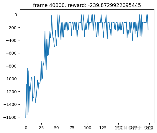
def plot(frame_idx, rewards):
    clear_output(True)
    plt.figure(figsize=(20,5))
    plt.subplot(131)
    plt.title('frame %s. reward: %s' % (frame_idx, rewards[-1]))
    plt.plot(rewards)
    plt.show()
class ValueNetwork(nn.Module):
    def __init__(self, state_dim, hidden_dim, init_w=3e-3):
        super(ValueNetwork, self).__init__()

        self.linear1 = nn.Linear(state_dim, hidden_dim)
        self.linear2 = nn.Linear(hidden_dim, hidden_dim)
        self.linear3 = nn.Linear(hidden_dim, 1)

        self.linear3.weight.data.uniform_(-init_w, init_w)
        self.linear3.bias.data.uniform_(-init_w, init_w)

    def forward(self, state):
        x = F.relu(self.linear1(state))
        x = F.relu(self.linear2(x))
        x = self.linear3(x)
        return x


class SoftQNetwork(nn.Module):
    def __init__(self, num_inputs, num_actions, hidden_size, init_w=3e-3):
        super(SoftQNetwork, self).__init__()

        self.linear1 = nn.Linear(num_inputs + num_actions, hidden_size)
        self.linear2 = nn.Linear(hidden_size, hidden_size)
        self.linear3 = nn.Linear(hidden_size, 1)

        self.linear3.weight.data.uniform_(-init_w, init_w)
        self.linear3.bias.data.uniform_(-init_w, init_w)

    def forward(self, state, action):
        x = torch.cat([state, action], 1)
        x = F.relu(self.linear1(x))
        x = F.relu(self.linear2(x))
        x = self.linear3(x)
        return x


class PolicyNetwork(nn.Module):
    def __init__(self, num_inputs, num_actions, hidden_size, init_w=3e-3, log_std_min=-20, log_std_max=2):
        super(PolicyNetwork, self).__init__()

        self.log_std_min = log_std_min
        self.log_std_max = log_std_max

        self.linear1 = nn.Linear(num_inputs, hidden_size)
        self.linear2 = nn.Linear(hidden_size, hidden_size)

        self.mean_linear = nn.Linear(hidden_size, num_actions)
        self.mean_linear.weight.data.uniform_(-init_w, init_w)
        self.mean_linear.bias.data.uniform_(-init_w, init_w)

        self.log_std_linear = nn.Linear(hidden_size, num_actions)
        self.log_std_linear.weight.data.uniform_(-init_w, init_w)
        self.log_std_linear.bias.data.uniform_(-init_w, init_w)

    def forward(self, state):
        x = F.relu(self.linear1(state))
        x = F.relu(self.linear2(x))

        mean    = self.mean_linear(x)
        log_std = self.log_std_linear(x)
        log_std = torch.clamp(log_std, self.log_std_min, self.log_std_max)

        return mean, log_std

    def evaluate(self, state, epsilon=1e-6):
        mean, log_std = self.forward(state)
        std = log_std.exp()

        normal = Normal(0, 1)
        z      = normal.sample()
        action = torch.tanh(mean+ std*z.to(device))
        # we sample some noise from a Standard Normal distribution and multiply it with our standard deviation,
        # and then add the result to the mean.
        log_prob = Normal(mean, std).log_prob(mean+ std*z.to(device)) - torch.log(1 - action.pow(2) + epsilon)
        return action, log_prob, z, mean, log_std


    def get_action(self, state):
        state = torch.FloatTensor(state).unsqueeze(0).to(device)
        mean, log_std = self.forward(state)
        std = log_std.exp()

        normal = Normal(0, 1)
        z      = normal.sample().to(device)
        action = torch.tanh(mean + std*z)

        action  = action.cpu()#.detach().cpu().numpy()
        return action[0]
#network update

def update(batch_size,gamma=0.99,soft_tau=1e-2,):

    state, action, reward, next_state, done = replay_buffer.sample(batch_size)

    state      = torch.FloatTensor(state).to(device)
    next_state = torch.FloatTensor(next_state).to(device)
    action     = torch.FloatTensor(action).to(device)
    reward     = torch.FloatTensor(reward).unsqueeze(1).to(device)
    done       = torch.FloatTensor(np.float32(done)).unsqueeze(1).to(device)

    predicted_q_value1 = soft_q_net1(state, action)
    predicted_q_value2 = soft_q_net2(state, action)
    predicted_value    = value_net(state)
    new_action, log_prob, epsilon, mean, log_std = policy_net.evaluate(state)


# Training Q Function
    target_value = target_value_net(next_state) #the predicted Q value for next state-action pair
    target_q_value = reward + (1 - done) * gamma * target_value #Bellman equation
    q_value_loss1 = soft_q_criterion1(predicted_q_value1, target_q_value.detach()) #reduce the MSE
    q_value_loss2 = soft_q_criterion2(predicted_q_value2, target_q_value.detach()) #reduce the MSE
    #.datch() method prevents gradient propagation

    soft_q_optimizer1.zero_grad()
    q_value_loss1.backward()
    soft_q_optimizer1.step()
    soft_q_optimizer2.zero_grad()
    q_value_loss2.backward()
    soft_q_optimizer2.step()

# Training Value Function
    predicted_new_q_value = torch.min(soft_q_net1(state, new_action),soft_q_net2(state, new_action)) #take the minimum of the two Q values
    target_value_func = predicted_new_q_value - log_prob #subtract from Policy’s log probability to select action in that state.
    value_loss = value_criterion(predicted_value, target_value_func.detach())

    value_optimizer.zero_grad()
    value_loss.backward()
    value_optimizer.step()

# Training Policy Function
    policy_loss = (log_prob - predicted_new_q_value).mean()

    policy_optimizer.zero_grad()
    policy_loss.backward()
    policy_optimizer.step()


    for target_param, param in zip(target_value_net.parameters(), value_net.parameters()):
        target_param.data.copy_(
            target_param.data * (1.0 - soft_tau) + param.data * soft_tau #determine update speed
        )
max_frames  = 40000
max_steps   = 500
frame_idx   = 0
rewards     = []
batch_size  = 128
#nested loops
#The outer loop initializes the environment for the beginning of the episode.
while frame_idx < max_frames:
    state = env.reset()
    episode_reward = 0

# Polyak averaging method
    for step in range(max_steps):
        if frame_idx >1000:
            action = policy_net.get_action(state).detach() #sample an action from the Policy network
            next_state, reward, done, _ = env.step(action.numpy())
        else:
            action = env.action_space.sample() #sample an action randomly from the action space for the first few time steps(1000)
            next_state, reward, done, _ = env.step(action)


        replay_buffer.push(state, action, reward, next_state, done)

        state = next_state
        episode_reward += reward
        frame_idx += 1

        if len(replay_buffer) > batch_size:
            update(batch_size)

        if frame_idx % 1000 == 0:
            plot(frame_idx, rewards)

        if done:
            break

    rewards.append(episode_reward)
from IPython.display import HTML
from matplotlib import animation

def display_frames_as_gif(frames):
    """
    Displays a list of frames as a gif, with controls
    """
    patch = plt.imshow(frames[0])
    plt.axis('off')

    def animate(i):
        patch.set_data(frames[i])

    anim = animation.FuncAnimation(plt.gcf(), animate, frames=len(frames), interval=50)
    return HTML(anim.to_jshtml())
import gym

env = gym.make("Pendulum-v1")

state = env.reset()
cum_reward = 0
frames = []
for t in range(50000):
    frames.append(env.render(mode='rgb_array'))
    action = policy_net.get_action(state)
    state, reward, done, info = env.step(action.detach().numpy())  # detach and convert to numpy
    reward = reward.item()  # convert reward from torch.Tensor to a float number
    cum_reward += reward
    if done:
        break
env.close()
display_frames_as_gif(frames)
结果如下:

小结
本文总结了学习SAC的过程,以倒立摆为例,从代码和算法理解两个角度入手解释。
感觉真的很有趣,从写代码的角度,和从理解SAC的运作过程的角度进行思考解释时,会得到不一样的顺序。


 794
794

 被折叠的 条评论
为什么被折叠?
被折叠的 条评论
为什么被折叠?
 到【灌水乐园】发言


