【机器学习】9.2.Tfidf 随机森林 朴素贝叶斯 自然语言处理 航空公司评论分类

包含全部示例的代码仓库见GIthub

1 导入库

import numpy as np
import pandas as pd
import re # 正则表达式
from sklearn.model_selection import train_test_split
from sklearn.feature_extraction.text import TfidfVectorizer
from sklearn.ensemble import RandomForestClassifier
from sklearn.model_selection import GridSearchCV
from sklearn.naive_bayes import MultinomialNB
from sklearn.metrics import classification_report
import pprint  # 打印
from sklearn.metrics import confusion_matrix
import matplotlib.pyplot as plt
%matplotlib inline

2 数据准备

data = pd.read_csv('./dataset/Tweets.csv')
data.head()
# output
tweet_id	airline_sentiment	airline_sentiment_confidence	negativereason	negativereason_confidence	airline	airline_sentiment_gold	name	negativereason_gold	retweet_count	text	tweet_coord	tweet_created	tweet_location	user_timezone
0	570306133677760513	neutral	1.0000	NaN	NaN	Virgin America	NaN	cairdin	NaN	0	@VirginAmerica What @dhepburn said.	NaN	2015-02-24 11:35:52 -0800	NaN	Eastern Time (US & Canada)
1	570301130888122368	positive	0.3486	NaN	0.0000	Virgin America	NaN	jnardino	NaN	0	@VirginAmerica plus you've added commercials t...	NaN	2015-02-24 11:15:59 -0800	NaN	Pacific Time (US & Canada)
2	570301083672813571	neutral	0.6837	NaN	NaN	Virgin America	NaN	yvonnalynn	NaN	0	@VirginAmerica I didn't today... Must mean I n...	NaN	2015-02-24 11:15:48 -0800	Lets Play	Central Time (US & Canada)
3	570301031407624196	negative	1.0000	Bad Flight	0.7033	Virgin America	NaN	jnardino	NaN	0	@VirginAmerica it's really aggressive to blast...	NaN	2015-02-24 11:15:36 -0800	NaN	Pacific Time (US & Canada)
4	570300817074462722	negative	1.0000	Can't Tell	1.0000	Virgin America	NaN	jnardino	NaN	0	@VirginAmerica and it's a really big bad thing...	NaN	2015-02-24 11:14:45 -0800	NaN	Pacific Time (US & Canada)

data = data[['airline_sentiment', 'text']]
data.info()
# output
<class 'pandas.core.frame.DataFrame'>
RangeIndex: 14640 entries, 0 to 14639
Data columns (total 2 columns):
 #   Column             Non-Null Count  Dtype 
---  ------             --------------  ----- 
 0   airline_sentiment  14640 non-null  object
 1   text               14640 non-null  object
dtypes: object(2)
memory usage: 228.9+ KB

data.airline_sentiment.unique()
# output
array(['neutral', 'positive', 'negative'], dtype=object)

data.airline_sentiment.value_counts()
# output
negative    9178
neutral     3099
positive    2363
Name: airline_sentiment, dtype: int64

树算法对处理不均匀数据效果较好，因此不做各类样本数量平衡

token = re.compile(r'[A-Za-z]+|[!?.:,()]')
def extract_text(text):
    new_text = token.findall(text)
    new_text = ' '.join([x.lower() for x in new_text]) # 变为小写，注意join前要有空格，否则会拼成一个单词
    return new_text
x = data.text.apply(extract_text)
y = data.airline_sentiment
x_train, x_test, y_train, y_test = train_test_split(x, y)
x_train.shape, x_test.shape
# output
((10980,), (3660,))

vect = TfidfVectorizer(ngram_range=(1,3), stop_words='english', min_df=3)
# (ngram_range=(1,3) 1-3个单词作为一个序列
x_train_vect = vect.fit_transform(x_train)  # 文本向量化
x_train_vect # 10980x361
x_test_vect = vect.transform(x_test)

3 模型构建_随机森林

model = RandomForestClassifier()
model.fit(x_train_vect, y_train)
model.score(x_train_vect, y_train)
# output
0.9934426229508196

model.score(x_test_vect, y_test)
# output
0.753551912568306

model2 = RandomForestClassifier(n_estimators=500)
model2.fit(x_train_vect, y_train)
model2.score(x_train_vect, y_train)
# output
0.9934426229508196

model2.score(x_test_vect, y_test)
# output
0.7543715846994535

交叉验证，搜索最优超参数

param = {
    'max_depth': range(1,500,10),
    'criterion': ['gini', 'entropy']
}
grid_s = GridSearchCV(RandomForestClassifier(n_jobs=8),
                      param_grid=param,
                      cv=5)
x_vect = vect.transform(x)  # 搜索最优超参数这里要transform一下，因为用全部数据做交叉验证
grid_s.fit(x_vect, y)

grid_s.best_estimator_
# output
RandomForestClassifier(criterion='entropy', max_depth=371, n_jobs=8)

grid_s.best_score_
# output
0.6948087431693989

4 模型构建_朴素贝叶斯

model = MultinomialNB(alpha=0.0001)
model.fit(x_train_vect, y_train)
model.score(x_train_vect, y_train)
# output
0.8883424408014572

model.score(x_test_vect, y_test)
# output
0.7502732240437159

超参数搜索
alpha平滑参数，越小越容易过拟合，越大越容易欠拟合

test_score = []
alpha = np.linspace(0.00001, 0.01, 100)  # 等距
for a in alpha:
    model = MultinomialNB(alpha=a)
    model.fit(x_train_vect, y_train)
    test_score.append(model.score(x_test_vect, y_test))
max_score = max(test_score)
max_score
# output
0.7573770491803279

index = test_score.index(max_score)
index
# output
94

alpha[index]
# output
0.009495454545454547

best_alpha = alpha[index]

5 模型评价

5.1 F1-Score

使用classification_report函数来查看针对每个类别的预测准确性

model = MultinomialNB(alpha=best_alpha)
model.fit(x_train_vect, y_train)
pred = model.predict(x_test_vect)
pprint.pprint(classification_report(y_test, pred))
# output
('              precision    recall  f1-score   support\n'
 '\n'
 '    negative       0.78      0.94      0.85      2288\n'
 '     neutral       0.63      0.38      0.47       781\n'
 '    positive       0.77      0.54      0.63       591\n'
 '\n'
 '    accuracy                           0.76      3660\n'
 '   macro avg       0.73      0.62      0.65      3660\n'
 'weighted avg       0.74      0.76      0.74      3660\n')

查准率 precision 召回率 recall
比如预测是否阳性
TP：将正类预测为正类数
FN：将正类预测为负类数
FP：将负类预测为正类数
TN：将负类预测为负类数
查准率 precision = TP/(TP+FP)
召回率 recall = TP/(TP+FN)
scikit-learn 评估性能的算法都在sklearn.metrics包里
查准率 sklearn.metrics.precision_score()
召回率 sklearn.metrics.recall_score()
F1-Score 同时兼顾了分类模型的精确率和召回率。F1-Score可以看作是模型准确率和召回率的一种加权平均

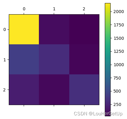
5.2 混淆矩阵

观察每一个类别被错误分类的情况，以矩阵形式将数据集中的记录按照真实的类别与分类模型预测的类别判断两个标准进行汇总。其中矩阵行表示真实值，列表示预测值。对角线上是预测正确的值。

cm = confusion_matrix(y_test, pred)
cm
# output
array([[2158,   99,   31],
       [ 422,  297,   62],
       [ 198,   76,  317]], dtype=int64)

plt.matshow(cm)
plt.colorbar()